library(PRcalc)
library(tidyverse)Measuring disproportionality
Preparation
data("jp_lower_2021_en")

# D'Hondt / Jefferson method
obj1 <- prcalc(jp_lower_2021_en,
               m = c(8, 13, 19, 22, 17, 11, 21, 28, 11, 6, 20),
               method = "dt")

# Hare-Niemeyer method
obj2 <- prcalc(jp_lower_2021_en,
               m = c(8, 13, 19, 22, 17, 11, 21, 28, 11, 6, 20),
               method = "hare")

# Sainte-Laguë / Webster method
obj3 <- prcalc(jp_lower_2021_en,
               m = c(8, 13, 19, 22, 17, 11, 21, 28, 11, 6, 20),
               method = "sl")

list("Jefferson" = obj1,
     "Hare"      = obj2,
     "Webster"   = obj3) |>
  compare() |>
print(use_gt = TRUE)| Party | Jefferson | Hare | Webster |
|---|---|---|---|
| LDP | 67 | 62 | 63 |
| NKP | 24 | 23 | 24 |
| CDP | 40 | 36 | 36 |
| JCP | 10 | 13 | 13 |
| JIP | 26 | 26 | 26 |
| DPP | 5 | 8 | 7 |
| SDP | 0 | 1 | 1 |
| Reiwa | 4 | 7 | 6 |
| NHK | 0 | 0 | 0 |
| SSN | 0 | 0 | 0 |
| JFP | 0 | 0 | 0 |
| Yamato | 0 | 0 | 0 |
| Corona | 0 | 0 | 0 |
Calculation of disproportionality indices.
- Some parameters are required for calculation of indices. Default is 2.
k:For Generalized Gallaghereta:For Atkinsonalpha:For \(\alpha\)-divergence
index1 <- index(obj1) # k = 2; eta = 2; alpha = 2
index1
ID Index Value
1 dhondt D’Hondt 1.13647
2 monroe Monroe 0.05321
3 maxdev Maximum Absolute Deviation 0.03413
4 mm_ratio Max-Min ratio Inf
5 rae Rae 0.01256
6 lh Loosemore & Hanby 0.08162
7 grofman Grofman 0.03335
8 lijphart Lijphart 0.03071
9 gallagher Gallagher 0.04129
10 g_gallagher Generalized Gallagher 0.04129
11 gatev Gatev 0.08744
12 ryabtsev Ryabtsev 0.06195
13 szalai Szalai 0.68738
14 w_szalai Weighted Szalai 0.15384
15 ap Aleskerov & Platonov 1.09773
16 gini Gini 0.07989
17 atkinson Atkinson 1.00000
18 sl Sainte-Laguë 0.05825
19 cs Cox & Shugart 1.13266
20 farina Farina 0.10153
21 ortona Ortona 0.12490
22 cd Cosine Dissimilarity 0.00417
23 rr Lebeda’s RR (Mixture D’Hondt) 0.12008
24 arr Lebeda’s ARR 0.00924
25 srr Lebeda’s SRR 0.04488
26 wdrr Lebeda’s WDRR 0.09444
27 kl Kullback-Leibler Surprise 0.04684
28 lr Likelihood Ratio Statistic Inf
29 chisq Chi Squared 0.03308
30 hellinger Hellinger Distance 0.14218
31 ad alpha-Divergence 0.02912index2 <- index(obj1, alpha = 1) # k = 2; eta = 2; alpha = 1
index2 ID Index Value
1 dhondt D’Hondt 1.13647
2 monroe Monroe 0.05321
3 maxdev Maximum Absolute Deviation 0.03413
4 mm_ratio Max-Min ratio Inf
5 rae Rae 0.01256
6 lh Loosemore & Hanby 0.08162
7 grofman Grofman 0.03335
8 lijphart Lijphart 0.03071
9 gallagher Gallagher 0.04129
10 g_gallagher Generalized Gallagher 0.04129
11 gatev Gatev 0.08744
12 ryabtsev Ryabtsev 0.06195
13 szalai Szalai 0.68738
14 w_szalai Weighted Szalai 0.15384
15 ap Aleskerov & Platonov 1.09773
16 gini Gini 0.07989
17 atkinson Atkinson 1.00000
18 sl Sainte-Laguë 0.05825
19 cs Cox & Shugart 1.13266
20 farina Farina 0.10153
21 ortona Ortona 0.12490
22 cd Cosine Dissimilarity 0.00417
23 rr Lebeda’s RR (Mixture D’Hondt) 0.12008
24 arr Lebeda’s ARR 0.00924
25 srr Lebeda’s SRR 0.04488
26 wdrr Lebeda’s WDRR 0.09444
27 kl Kullback-Leibler Surprise 0.04684
28 lr Likelihood Ratio Statistic Inf
29 chisq Chi Squared 0.03308
30 hellinger Hellinger Distance 0.14218
31 ad alpha-Divergence 0.04684Printing
You can extract specific indices using [ operator.
# Extract Gallagher index.
index1["gallagher"]
gallagher
0.04128719 # Extract Gallagher index and alpha-divergence.
index1[c("gallagher", "ad")] gallagher ad
0.04128719 0.02912491 The identifiers for each indicator are as follows:
Error in gt(tibble(ID = attr(index1, "names"), Name = attr(index1, "labels"))): could not find function "gt"The subset argument of print() function can be used to output the result in a tabular format.
# Extract a subset of indices.
print(index1, subset = c("dhondt", "gallagher", "lh", "ad"))
ID Index Value
1 dhondt D’Hondt 1.1365
2 lh Loosemore & Hanby 0.0816
3 gallagher Gallagher 0.0413
4 ad alpha-Divergence 0.0291The hide_id argument can also be used to hide the ID column.
# Hide ID column.
print(index1,
      subset  = c("dhondt", "gallagher", "lh", "ad"),
      hide_id = TRUE)
Index Value
1 D’Hondt 1.1365
2 Loosemore & Hanby 0.0816
3 Gallagher 0.0413
4 alpha-Divergence 0.0291The use_gt argument can be used to print results using {gt} package.
# Use {gt} package
print(index2,
      subset  = c("dhondt", "gallagher", "lh", "ad"),
      hide_id = TRUE,
use_gt = TRUE)| Index | Value |
|---|---|
| D’Hondt | 1.136 |
| Loosemore & Hanby | 0.082 |
| Gallagher | 0.041 |
| alpha-Divergence | 0.047 |
Visulaization
plot(index2)Don't know how to automatically pick scale for object of type <prcalc_index>.
Defaulting to continuous.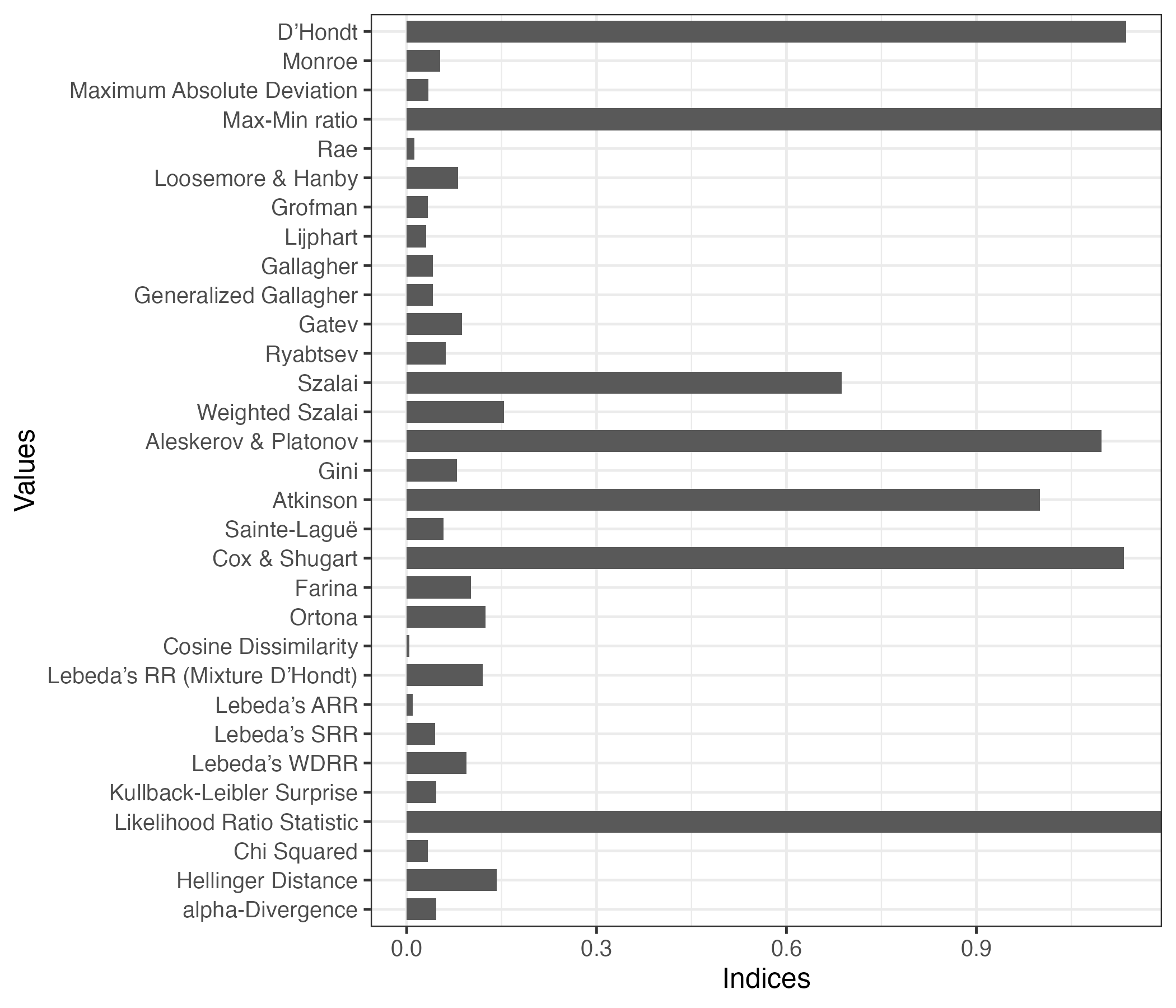
plot(index2, style = "lollipop") # lollipop chartDon't know how to automatically pick scale for object of type <prcalc_index>.
Defaulting to continuous.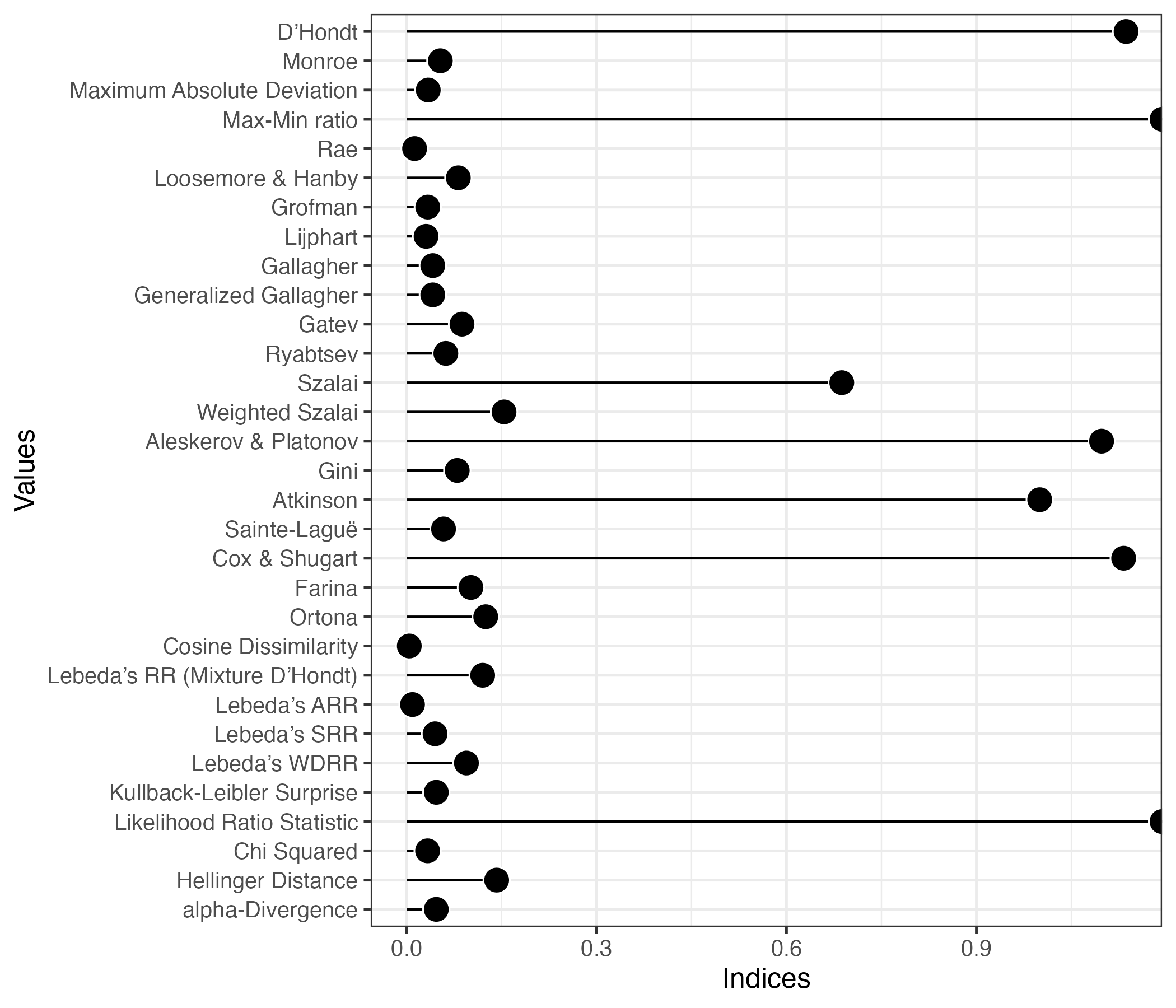
plot(index2, index = c("dhondt", "gallagher", "lh", "ad"))Don't know how to automatically pick scale for object of type <prcalc_index>.
Defaulting to continuous.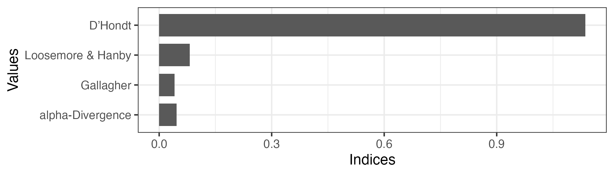
Comparison
compare(list(index(obj1), index(obj2), index(obj3))) ID Index Model1 Model2 Model3
1 dhondt D’Hondt 1.13647 1.055589 1.10148
2 monroe Monroe 0.05321 0.020396 0.02505
3 maxdev Maximum Absolute Deviation 0.03413 0.013865 0.01387
4 mm_ratio Max-Min ratio Inf Inf Inf
5 rae Rae 0.01256 0.004263 0.00577
6 lh Loosemore & Hanby 0.08162 0.027708 0.03753
7 grofman Grofman 0.03335 0.011323 0.01534
8 lijphart Lijphart 0.03071 0.005143 0.00798
9 gallagher Gallagher 0.04129 0.015827 0.01944
10 g_gallagher Generalized Gallagher 0.04129 0.015827 0.01944
11 gatev Gatev 0.08744 0.034607 0.04227
12 ryabtsev Ryabtsev 0.06195 0.024478 0.02990
13 szalai Szalai 0.68738 0.636499 0.63706
14 w_szalai Weighted Szalai 0.15384 0.105784 0.10847
15 ap Aleskerov & Platonov 1.09773 1.029574 1.04611
16 gini Gini 0.07989 0.032180 0.04213
17 atkinson Atkinson 1.00000 1.000000 1.00000
18 sl Sainte-Laguë 0.05825 0.024911 0.02720
19 cs Cox & Shugart 1.13266 1.035874 1.05312
20 farina Farina 0.10153 0.047980 0.05482
21 ortona Ortona 0.12490 0.042402 0.05743
22 cd Cosine Dissimilarity 0.00417 0.000932 0.00122
23 rr Lebeda’s RR (Mixture D’Hondt) 0.12008 0.052662 0.09213
24 arr Lebeda’s ARR 0.00924 0.004051 0.00709
25 srr Lebeda’s SRR 0.04488 0.023669 0.03500
26 wdrr Lebeda’s WDRR 0.09444 0.036026 0.05573
27 kl Kullback-Leibler Surprise 0.04684 0.021767 0.02292
28 lr Likelihood Ratio Statistic Inf Inf Inf
29 chisq Chi Squared 0.03308 0.026543 0.02888
30 hellinger Hellinger Distance 0.14218 0.098133 0.09959
31 ad alpha-Divergence 0.02912 0.012455 0.01360compare(list("D'Hondt" = index(obj1),
"Hare" = index(obj2),
"Sainte-Laguë" = index(obj3))) ID Index D'Hondt Hare Sainte-Laguë
1 dhondt D’Hondt 1.13647 1.055589 1.10148
2 monroe Monroe 0.05321 0.020396 0.02505
3 maxdev Maximum Absolute Deviation 0.03413 0.013865 0.01387
4 mm_ratio Max-Min ratio Inf Inf Inf
5 rae Rae 0.01256 0.004263 0.00577
6 lh Loosemore & Hanby 0.08162 0.027708 0.03753
7 grofman Grofman 0.03335 0.011323 0.01534
8 lijphart Lijphart 0.03071 0.005143 0.00798
9 gallagher Gallagher 0.04129 0.015827 0.01944
10 g_gallagher Generalized Gallagher 0.04129 0.015827 0.01944
11 gatev Gatev 0.08744 0.034607 0.04227
12 ryabtsev Ryabtsev 0.06195 0.024478 0.02990
13 szalai Szalai 0.68738 0.636499 0.63706
14 w_szalai Weighted Szalai 0.15384 0.105784 0.10847
15 ap Aleskerov & Platonov 1.09773 1.029574 1.04611
16 gini Gini 0.07989 0.032180 0.04213
17 atkinson Atkinson 1.00000 1.000000 1.00000
18 sl Sainte-Laguë 0.05825 0.024911 0.02720
19 cs Cox & Shugart 1.13266 1.035874 1.05312
20 farina Farina 0.10153 0.047980 0.05482
21 ortona Ortona 0.12490 0.042402 0.05743
22 cd Cosine Dissimilarity 0.00417 0.000932 0.00122
23 rr Lebeda’s RR (Mixture D’Hondt) 0.12008 0.052662 0.09213
24 arr Lebeda’s ARR 0.00924 0.004051 0.00709
25 srr Lebeda’s SRR 0.04488 0.023669 0.03500
26 wdrr Lebeda’s WDRR 0.09444 0.036026 0.05573
27 kl Kullback-Leibler Surprise 0.04684 0.021767 0.02292
28 lr Likelihood Ratio Statistic Inf Inf Inf
29 chisq Chi Squared 0.03308 0.026543 0.02888
30 hellinger Hellinger Distance 0.14218 0.098133 0.09959
31 ad alpha-Divergence 0.02912 0.012455 0.01360compare(list("D'Hondt" = index(obj1),
"Hare" = index(obj2),
"Sainte-Laguë" = index(obj3)))|>
print(hide_id = TRUE) Index D'Hondt Hare Sainte-Laguë
1 D’Hondt 1.13647 1.055589 1.10148
2 Monroe 0.05321 0.020396 0.02505
3 Maximum Absolute Deviation 0.03413 0.013865 0.01387
4 Max-Min ratio Inf Inf Inf
5 Rae 0.01256 0.004263 0.00577
6 Loosemore & Hanby 0.08162 0.027708 0.03753
7 Grofman 0.03335 0.011323 0.01534
8 Lijphart 0.03071 0.005143 0.00798
9 Gallagher 0.04129 0.015827 0.01944
10 Generalized Gallagher 0.04129 0.015827 0.01944
11 Gatev 0.08744 0.034607 0.04227
12 Ryabtsev 0.06195 0.024478 0.02990
13 Szalai 0.68738 0.636499 0.63706
14 Weighted Szalai 0.15384 0.105784 0.10847
15 Aleskerov & Platonov 1.09773 1.029574 1.04611
16 Gini 0.07989 0.032180 0.04213
17 Atkinson 1.00000 1.000000 1.00000
18 Sainte-Laguë 0.05825 0.024911 0.02720
19 Cox & Shugart 1.13266 1.035874 1.05312
20 Farina 0.10153 0.047980 0.05482
21 Ortona 0.12490 0.042402 0.05743
22 Cosine Dissimilarity 0.00417 0.000932 0.00122
23 Lebeda’s RR (Mixture D’Hondt) 0.12008 0.052662 0.09213
24 Lebeda’s ARR 0.00924 0.004051 0.00709
25 Lebeda’s SRR 0.04488 0.023669 0.03500
26 Lebeda’s WDRR 0.09444 0.036026 0.05573
27 Kullback-Leibler Surprise 0.04684 0.021767 0.02292
28 Likelihood Ratio Statistic Inf Inf Inf
29 Chi Squared 0.03308 0.026543 0.02888
30 Hellinger Distance 0.14218 0.098133 0.09959
31 alpha-Divergence 0.02912 0.012455 0.01360compare(list("D'Hondt" = index(obj1),
"Hare" = index(obj2),
"Sainte-Laguë" = index(obj3))) |>
print(subset = c("dhondt", "gallagher", "lh", "ad"),
hide_id = TRUE,
use_gt = TRUE)| Index | D'Hondt | Hare | Sainte-Laguë |
|---|---|---|---|
| D’Hondt | 1.136 | 1.056 | 1.101 |
| Loosemore & Hanby | 0.082 | 0.028 | 0.038 |
| Gallagher | 0.041 | 0.016 | 0.019 |
| alpha-Divergence | 0.029 | 0.012 | 0.014 |
compare(list("D'Hondt"      = index(obj1),
             "Hare"         = index(obj2),
"Sainte-Laguë" = index(obj3))) |>
plot() +
ggplot2::labs(x = "Values", y = "Indices", fill = "Method")Don't know how to automatically pick scale for object of type <prcalc_index>.
Defaulting to continuous.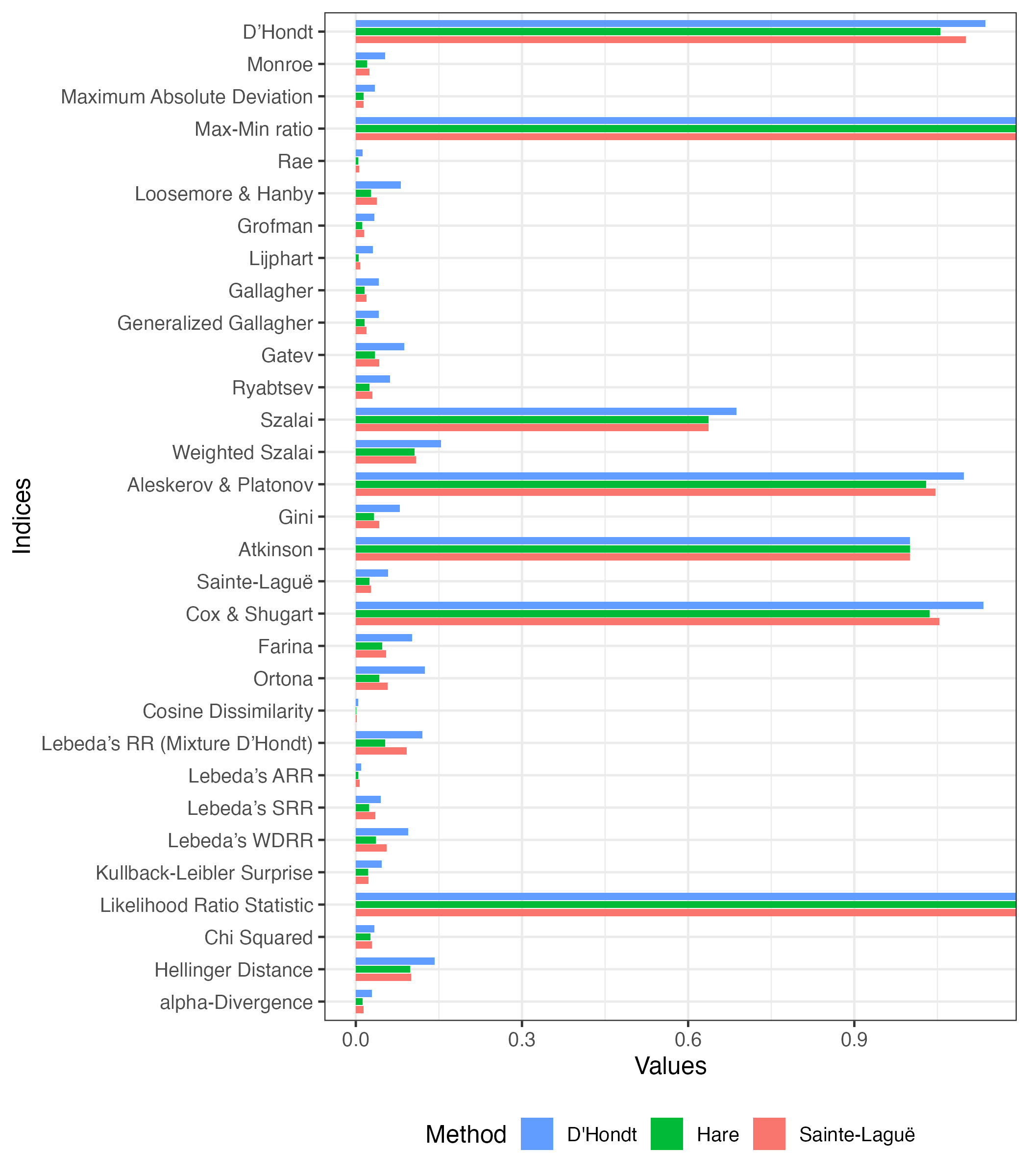
Marginal and joint distribution
For illustration purposes, we extract some parties and districts from jp_lower_2021_en and allocate seats.
tiny_data <- jp_lower_2021_en |>
  filter(Party %in% c("LDP", "NKP", "CDP", "JCP", "JIP")) |>
  select(Party, Tokyo, Tokai, Kinki, Kyushu)

tiny_obj <- prcalc(tiny_data, m = c(30, 20, 40, 20), method = "dt")
tiny_obj
Raw:
Party Tokyo Tokai Kinki Kyushu Total
1 LDP 2000084 2515841 2407699 2250966 9174590
2 NKP 715450 784976 1155683 1040756 3696865
3 CDP 1293281 1485947 1090666 1266801 5136695
4 JCP 670340 408606 736156 365658 2180760
5 JIP 858577 694630 3180219 540338 5273764
Result:
Party Tokyo Tokai Kinki Kyushu Total
1 LDP 11 9 12 8 40
2 NKP 4 3 5 4 16
3 CDP 7 5 5 5 22
4 JCP 3 1 3 1 8
5 JIP 5 2 15 2 24
Parameters:
Allocation method: D'Hondt (Jefferson) method
Extra parameter:
Threshold: 0
Magnitude:
Tokyo Tokai Kinki Kyushu
30 20 40 20 index(tiny_obj)["ad"] ad
0.001292773 Calculating \(\alpha\)-diveregen from tiny_obj yields a result of 0.00129 (\(\alpha\) = 2). Disproportionality is calculated based on the number of votes and seats. However, if the same party spans multiple districts, the results will vary depending on how votes and seats are defined. {PRcalc} defines the number of votes and seats obtained using the marginal or simultaneous distribution of the vote and seat matrices.
Using marginal distribution of rows
When parties (level 2) span districts (level 1), as in tiny_obj, the marginal distribution of rows (level 2) can be used as the number of votes and seats. That is, the sum of the votes and seats won by each party in each district is used.
| Party | Tokyo | Tokai | Kinki | Kyushu | Total |
|---|---|---|---|---|---|
| LDP | 2000084 | 2515841 | 2407699 | 2250966 | 9174590 |
| NKP | 715450 | 784976 | 1155683 | 1040756 | 3696865 |
| CDP | 1293281 | 1485947 | 1090666 | 1266801 | 5136695 |
| JCP | 670340 | 408606 | 736156 | 365658 | 2180760 |
| JIP | 858577 | 694630 | 3180219 | 540338 | 5273764 |
| Total | 5537732 | 5890000 | 8570423 | 5464519 | 25462674 |
| Party | Tokyo | Tokai | Kinki | Kyushu | Total |
|---|---|---|---|---|---|
| LDP | 11 | 9 | 12 | 8 | 40 |
| NKP | 4 | 3 | 5 | 4 | 16 |
| CDP | 7 | 5 | 5 | 5 | 22 |
| JCP | 3 | 1 | 3 | 1 | 8 |
| JIP | 5 | 2 | 15 | 2 | 24 |
| Total | 30 | 20 | 40 | 20 | 110 |
| Party | Vote | Seat |
|---|---|---|
| LDP | 9174590 | 40 |
| NKP | 3696865 | 16 |
| CDP | 5136695 | 22 |
| JCP | 2180760 | 8 |
| JIP | 5273764 | 24 |
Use the peripheral distribution of rows by setting unit = "l2", which is the default.
index(tiny_obj, unit = "l2")["ad"] ad
0.001292773 However, if level 2 is completely nested instead of spanning level 1, then the marginalization of level 2 is meaningless. In this case, we recommend peripheral distribution of level 1 ("l1") or joint distribution ("joint").
Using marginal distribution of columns
If unit = "l1", the marginal distribution of column (level 1; in this example, district) is used as the number of votes and seats.
| Party | Tokyo | Tokai | Kinki | Kyushu | Total |
|---|---|---|---|---|---|
| LDP | 2000084 | 2515841 | 2407699 | 2250966 | 9174590 |
| NKP | 715450 | 784976 | 1155683 | 1040756 | 3696865 |
| CDP | 1293281 | 1485947 | 1090666 | 1266801 | 5136695 |
| JCP | 670340 | 408606 | 736156 | 365658 | 2180760 |
| JIP | 858577 | 694630 | 3180219 | 540338 | 5273764 |
| Total | 5537732 | 5890000 | 8570423 | 5464519 | 25462674 |
| Party | Tokyo | Tokai | Kinki | Kyushu | Total |
|---|---|---|---|---|---|
| LDP | 11 | 9 | 12 | 8 | 40 |
| NKP | 4 | 3 | 5 | 4 | 16 |
| CDP | 7 | 5 | 5 | 5 | 22 |
| JCP | 3 | 1 | 3 | 1 | 8 |
| JIP | 5 | 2 | 15 | 2 | 24 |
| Total | 30 | 20 | 40 | 20 | 110 |
| Party | Vote | Seat |
|---|---|---|
| Tokyo | 5537732 | 30 |
| Tokai | 5890000 | 20 |
| Kinki | 8570423 | 40 |
| Kyushu | 5464519 | 20 |
index(tiny_obj, unit = "l1")["ad"] ad
0.01590448 The \(\alpha\)-divergence in the case of marginalization in district matches the value of reapportionment-stage in decomposition.
Using joint distritubion
If unit = "joint", the votes and seats won by each party in their respective districts are used as is.
| Party | Tokyo | Tokai | Kinki | Kyushu | Total |
|---|---|---|---|---|---|
| LDP | 2000084 | 2515841 | 2407699 | 2250966 | 9174590 |
| NKP | 715450 | 784976 | 1155683 | 1040756 | 3696865 |
| CDP | 1293281 | 1485947 | 1090666 | 1266801 | 5136695 |
| JCP | 670340 | 408606 | 736156 | 365658 | 2180760 |
| JIP | 858577 | 694630 | 3180219 | 540338 | 5273764 |
| Total | 5537732 | 5890000 | 8570423 | 5464519 | 25462674 |
| Party | Tokyo | Tokai | Kinki | Kyushu | Total |
|---|---|---|---|---|---|
| LDP | 11 | 9 | 12 | 8 | 40 |
| NKP | 4 | 3 | 5 | 4 | 16 |
| CDP | 7 | 5 | 5 | 5 | 22 |
| JCP | 3 | 1 | 3 | 1 | 8 |
| JIP | 5 | 2 | 15 | 2 | 24 |
| Total | 30 | 20 | 40 | 20 | 110 |
| Party_Pref | Vote | Seat |
|---|---|---|
| LDP_Tokyo | 2000084 | 11 |
| LDP_Tokai | 2515841 | 9 |
| LDP_Kinki | 2407699 | 12 |
| LDP_Kyushu | 2250966 | 8 |
| NKP_Tokyo | 715450 | 4 |
| NKP_Tokai | 784976 | 3 |
| NKP_Kinki | 1155683 | 5 |
| NKP_Kyushu | 1040756 | 4 |
| CDP_Tokyo | 1293281 | 7 |
| CDP_Tokai | 1485947 | 5 |
| CDP_Kinki | 1090666 | 5 |
| CDP_Kyushu | 1266801 | 5 |
| JCP_Tokyo | 670340 | 3 |
| JCP_Tokai | 408606 | 1 |
| JCP_Kinki | 736156 | 3 |
| JCP_Kyushu | 365658 | 1 |
| JIP_Tokyo | 858577 | 5 |
| JIP_Tokai | 694630 | 2 |
| JIP_Kinki | 3180219 | 15 |
| JIP_Kyushu | 540338 | 2 |
index(tiny_obj, unit = "joint")["ad"] ad
0.01872325 index() and decompose()
decompose(tiny_obj)alpha = 2
alpha-divergence Reapportionment Redistricting
0.01872325 0.01590448 0.00281877
Note: "alha-divergence" is sum of "Reapportionment" and "Redisticting" terms.The \(\alpha\)-divergence in the case of marginalization in district (unit = "l1") matches the value of reapportionment-stage in decomposition.
index(tiny_obj, unit = "l1")["ad"] ad
0.01590448 The \(\alpha\)-divergence based on joint distribution (unit = "joint") is consistent with \(\alpha\)-divergence in decomposition.
index(tiny_obj, unit = "joint")["ad"] ad
0.01872325