差分の差分法

スライド

セットアップ

　本日の実習に必要なパッケージとデータを読み込む。

pacman::p_load(tidyverse,     # Rの必須パッケージ
               summarytools,  # 記述統計
               modelsummary,  # 推定結果の要約
               estimatr,      # ロバストな回帰分析
               gsynth,        # 一般化SCM
               panelView)     # パネルデータのチェック

did_df <- read_csv("data/did_data4.csv")

did_df

# A tibble: 18,749 × 14
   county state  year shooting fatal_shooting non_fatal_shooting turnout demvote
    <dbl> <chr> <dbl>    <dbl>          <dbl>              <dbl>   <dbl>   <dbl>
 1   1001 01     1996        0              0                  0    56.1    32.5
 2   1001 01     2000        0              0                  0    56.8    28.7
 3   1001 01     2004        0              0                  0    60.2    23.7
 4   1001 01     2008        0              0                  0    64.1    25.8
 5   1001 01     2012        0              0                  0    61.0    26.5
 6   1001 01     2016        0              0                  0    60.7    24.0
 7   1003 01     1996        0              0                  0    51.8    27.1
 8   1003 01     2000        0              0                  0    54.6    24.8
 9   1003 01     2004        0              0                  0    59.8    22.5
10   1003 01     2008        0              0                  0    62.4    23.8
# ℹ 18,739 more rows
# ℹ 6 more variables: population <dbl>, non_white <dbl>,
#   change_unem_rate <dbl>, county_f <dbl>, state_f <chr>, year_f <dbl>

　データの詳細はスライドを参照すること。DID推定には時間（年）とカウンティー（郡）の固定効果を投入し、州レベルでクラスタリングした標準誤差を使う予定である。これらの変数を予めfactor化しておこう。factor化した変数は変数名の後ろに_fを付けて、新しい列として追加しておく。

did_df <- did_df |>
  mutate(county_f = factor(county),
         state_f  = factor(state),
         year_f   = factor(year))

did_df

# A tibble: 18,749 × 14
   county state  year shooting fatal_shooting non_fatal_shooting turnout demvote
    <dbl> <chr> <dbl>    <dbl>          <dbl>              <dbl>   <dbl>   <dbl>
 1   1001 01     1996        0              0                  0    56.1    32.5
 2   1001 01     2000        0              0                  0    56.8    28.7
 3   1001 01     2004        0              0                  0    60.2    23.7
 4   1001 01     2008        0              0                  0    64.1    25.8
 5   1001 01     2012        0              0                  0    61.0    26.5
 6   1001 01     2016        0              0                  0    60.7    24.0
 7   1003 01     1996        0              0                  0    51.8    27.1
 8   1003 01     2000        0              0                  0    54.6    24.8
 9   1003 01     2004        0              0                  0    59.8    22.5
10   1003 01     2008        0              0                  0    62.4    23.8
# ℹ 18,739 more rows
# ℹ 6 more variables: population <dbl>, non_white <dbl>,
#   change_unem_rate <dbl>, county_f <fct>, state_f <fct>, year_f <fct>

　連続変数（shootingからchange_unem_rateまで）の記述統計量を出力する。

did_df |>
  select(shooting:change_unem_rate) |>
  descr(stats = c("mean", "sd", "min", "max", "n.valid"),
        transpose = TRUE, order = "p")

Descriptive Statistics  

                               Mean     Std.Dev      Min           Max    N.Valid
------------------------ ---------- ----------- -------- ------------- ----------
                shooting       0.00        0.07     0.00          1.00   18749.00
          fatal_shooting       0.00        0.05     0.00          1.00   18749.00
      non_fatal_shooting       0.00        0.04     0.00          1.00   18749.00
                 turnout      57.94       10.32     1.08        300.00   18627.00
                 demvote      39.01       13.79     3.14         92.85   18627.00
              population   95121.69   306688.63    55.00   10137915.00   18749.00
               non_white       0.13        0.16     0.00          0.96   18749.00
        change_unem_rate      -0.39        2.34   -19.60         15.30   18749.00

select()関数がおかしい?

　今回の講義に限らず、よくある問題としてパッケージ間の衝突がある。これは同じ名前の関数が複数存在する際に生じる。たとえば、select()関数は{dplyr}パッケージだけでなく、{MASS}という有名なパッケージにも同じ名前の関数が存在する。自分が{dplyr}のみ読み込み、{MASS}を読み込まなかったとしても衝突は生じうる。たとえば、{X}というパッケージが{MASS}に依存する場合、{X}を読み込むと、裏では{MASS}も読み込まれるからだ。そもそも我々も{dplyr}を読み込んでないが、{tidyverse}が{dplyr}に依存しているため、{dplyr}が読み込まれている。

　したがって、絶対存在するはずの関数で使い方も間違っていないにも関わらずエラーが発生した場合は、「どのパッケージの関数か」を明記してみよう。書き方はパッケージ名::関数名()だ。たとえば、{dplyr}パッケージのselect()関数はdplyr::select()と書く。

Diff-in-Diff

　それでは差分の差分法の実装について紹介する。推定式は以下の通りである。

\[ \mbox{Outcome}_{i, t} = \beta_0 + \beta_1 \mbox{Shooting}_{i, t} + \sum_k \delta_{k, i, t} \mbox{Controls}_{k, i, t} + \lambda_{t} + \omega_{i} + \varepsilon_{i, t} \]

$\mbox{Otucome}$: 応答変数
- turnout: 投票率（大統領選挙）
- demvote: 民主党候補者の得票率
$\mbox{Shooting}$: 処置変数
- shooting: 銃撃事件の発生有無
- fatal_shooting: 死者を伴う銃撃事件の発生有無
- non_fatal_shooting: 死者を伴わない銃撃事件の発生有無
$\mbox{Controls}$: 統制変数
- population: カウンティーの人口
- non_white: 非白人の割合
- change_unem_rate: 失業率の変化
- 統制変数あり/なしのモデルを個別に推定
$\lambda$: 年固定効果
$\omega$: カウンティー固定効果

応答変数が2種類、処置変数が3種類、共変量の有無でモデルを分けるので、推定するモデルは計12個である。

モデル	オブジェクト名	応答変数	処置変数	統制変数
モデル1	`did_fit1`	`turnout`	`shooting`	なし
モデル2	`did_fit2`	`turnout`	`shooting`	あり
モデル3	`did_fit3`	`turnout`	`fatal_shooting`	なし
モデル4	`did_fit4`	`turnout`	`fatal_shooting`	あり
モデル5	`did_fit5`	`turnout`	`non_fatal_shooting`	なし
モデル6	`did_fit6`	`turnout`	`non_fatal_shooting`	あり
モデル7	`did_fit7`	`demvote`	`shooting`	なし
モデル8	`did_fit8`	`demvote`	`shooting`	あり
モデル9	`did_fit9`	`demvote`	`fatal_shooting`	なし
モデル10	`did_fit10`	`demvote`	`fatal_shooting`	あり
モデル11	`did_fit11`	`demvote`	`non_fatal_shooting`	なし
モデル12	`did_fit12`	`demvote`	`non_fatal_shooting`	あり

　まずはモデル1を推定し、did_fit1という名のオブジェクトとして格納する。基本的には線形回帰分析であるため、lm()でも推定はできる。しかし、差分の差分法の場合、通常、クラスター化した頑健な標準誤差（cluster robust standard error）を使う。lm()単体ではこれが計算できないため、今回は{estimatr}パッケージが提供するlm_robust()関数を使用する。使い方はlm()同様、まず回帰式と使用するデータ名を指定する。続いて、固定効果をfixed_effects引数で指定する¹。書き方は~固定効果変数1 + 固定効果変数2 + ...である。回帰式と違って、~の左側には変数がないことに注意すること。続いて、clusters引数でクラスタリングする変数を指定する。今回は州レベルでクラスタリングするので、state_fで良い。最後に標準誤差のタイプを指定するが、デフォルトは"CR2"となっている。今回のデータはそれなりの大きさのデータであり、"CR2"だと推定時間が非常に長くなる。ここでは推定時間が比較的早い"stata"とする。

did_fit1 <- lm_robust(turnout ~ shooting, 
                      data          = did_df, 
                      fixed_effects = ~year_f + county_f,
                      clusters      = state_f,
                      se_type       = "stata")

summary(did_fit1)


Call:
lm_robust(formula = turnout ~ shooting, data = did_df, clusters = state_f, 
    fixed_effects = ~year_f + county_f, se_type = "stata")

Standard error type:  stata 

Coefficients:
         Estimate Std. Error t value Pr(>|t|) CI Lower CI Upper DF
shooting  -0.5211     0.6457  -0.807   0.4235   -1.819   0.7764 49

Multiple R-squared:  0.8575 ,   Adjusted R-squared:  0.8288
Multiple R-squared (proj. model):  6.907e-05 ,  Adjusted R-squared (proj. model):  -0.2008 
F-statistic (proj. model): 0.6513 on 1 and 49 DF,  p-value: 0.4235

　処置効果の推定値は-0.521である。これは学校内銃撃事件が発生したカウンティーの場合、大統領選挙において投票率が約-0.521%p低下することを意味する。しかし、標準誤差がかなり大きく、統計的有意な結果ではない。つまり、「学校内銃撃事件が投票率を上げる（or 下げる）とは言えない」と解釈できる。決して「学校内銃撃事件が投票率を上げない（or 下げない）」と解釈しないこと。

　共変量を投入してみたらどうだろうか。たとえば、人口は自治体の都市化程度を表すこともあるので、都市化程度と投票率には関係があると考えられる。また、人口が多いと自然に事件が発生する確率もあがるので、交絡要因として考えられる。人種や失業率も同様であろう。ここではカウンティーの人口（population）、非白人の割合（non_white）、失業率の変化（change_unem_rate）を統制変数として投入し、did_fit2という名で格納する。

did_fit2 <- lm_robust(turnout ~ shooting + 
                        population + non_white + change_unem_rate, 
                      data          = did_df, 
                      fixed_effects = ~year_f + county_f,
                      clusters      = state_f,
                      se_type       = "stata")

summary(did_fit2)


Call:
lm_robust(formula = turnout ~ shooting + population + non_white + 
    change_unem_rate, data = did_df, clusters = state_f, fixed_effects = ~year_f + 
    county_f, se_type = "stata")

Standard error type:  stata 

Coefficients:
                   Estimate Std. Error t value Pr(>|t|)   CI Lower   CI Upper
shooting         -7.098e-01  6.237e-01  -1.138  0.26066 -1.963e+00  5.436e-01
population        8.029e-06  5.688e-06   1.411  0.16443 -3.402e-06  1.946e-05
non_white        -3.483e+01  1.558e+01  -2.236  0.02990 -6.613e+01 -3.534e+00
change_unem_rate  1.592e-01  6.584e-02   2.418  0.01938  2.688e-02  2.915e-01
                 DF
shooting         49
population       49
non_white        49
change_unem_rate 49

Multiple R-squared:  0.8598 ,   Adjusted R-squared:  0.8316
Multiple R-squared (proj. model):  0.01669 ,    Adjusted R-squared (proj. model):  -0.1811 
F-statistic (proj. model): 5.047 on 4 and 49 DF,  p-value: 0.001739

　処置効果の推定値は-0.710である。これは他の条件が同じ場合、学校内銃撃事件が発生したカウンティーは大統領選挙において投票率が約-0.710%p低下することを意味する。ちなみに、e-01は$\times 10^{-1}$を、e-06は$\times 10^{-6}$を、e+01は$\times 10^{1}$意味する。今回も統計的に非有意な結果が得られている。

　これまでの処置変数は死者の有無と関係なく、学校内銃撃事件が発生したか否かだった。もしかしたら、死者を伴う銃撃事件が発生した場合、その効果が大きいかも知れない。したがって、これからは処置変数を死者を伴う学校内銃撃事件の発生有無（fatal_shooting）、死者を伴わない学校内銃撃事件の発生有無（non_fatal_shooting）に変えてもう一度推定してみよう。

did_fit3 <- lm_robust(turnout ~ fatal_shooting, 
                      data          = did_df, 
                      fixed_effects = ~year_f + county_f,
                      clusters      = state_f,
                      se_type       = "stata")

did_fit4 <- lm_robust(turnout ~ fatal_shooting + 
                        population + non_white + change_unem_rate, 
                      data          = did_df, 
                      fixed_effects = ~year_f + county_f,
                      clusters      = state_f,
                      se_type       = "stata")

did_fit5 <- lm_robust(turnout ~ non_fatal_shooting, 
                      data          = did_df, 
                      fixed_effects = ~year_f + county_f,
                      clusters      = state_f,
                      se_type       = "stata")

did_fit6 <- lm_robust(turnout ~ non_fatal_shooting + 
                        population + non_white + change_unem_rate, 
                      data          = did_df, 
                      fixed_effects = ~year_f + county_f,
                      clusters      = state_f,
                      se_type       = "stata")

　これまで推定してきた6つのモデルを比較してみよう。

modelsummary(list(did_fit1, did_fit2, did_fit3, 
                  did_fit4, did_fit5, did_fit6))

	(1)	(2)	(3)	(4)	(5)	(6)
shooting	−0.521	−0.710
	(0.646)	(0.624)
population		0.000		0.000		0.000
		(0.000)		(0.000)		(0.000)
non_white		−34.834		−34.844		−34.814
		(15.575)		(15.618)		(15.614)
change_unem_rate		0.159		0.159		0.160
		(0.066)		(0.066)		(0.066)
fatal_shooting			−0.678	−0.918
			(0.619)	(0.658)
non_fatal_shooting					−0.239	−0.327
					(1.094)	(1.145)
Num.Obs.	18627	18627	18627	18627	18627	18627
R2	0.857	0.860	0.857	0.860	0.857	0.860
R2 Adj.	0.829	0.832	0.829	0.832	0.829	0.832
AIC	103543.4	103237.2	103543.3	103237.1	103544.6	103239.4
BIC	103559.0	103276.4	103559.0	103276.3	103560.2	103278.6
RMSE	3.90	3.87	3.90	3.87	3.90	3.87
Std.Errors	by: state_f	by: state_f	by: state_f	by: state_f	by: state_f	by: state_f

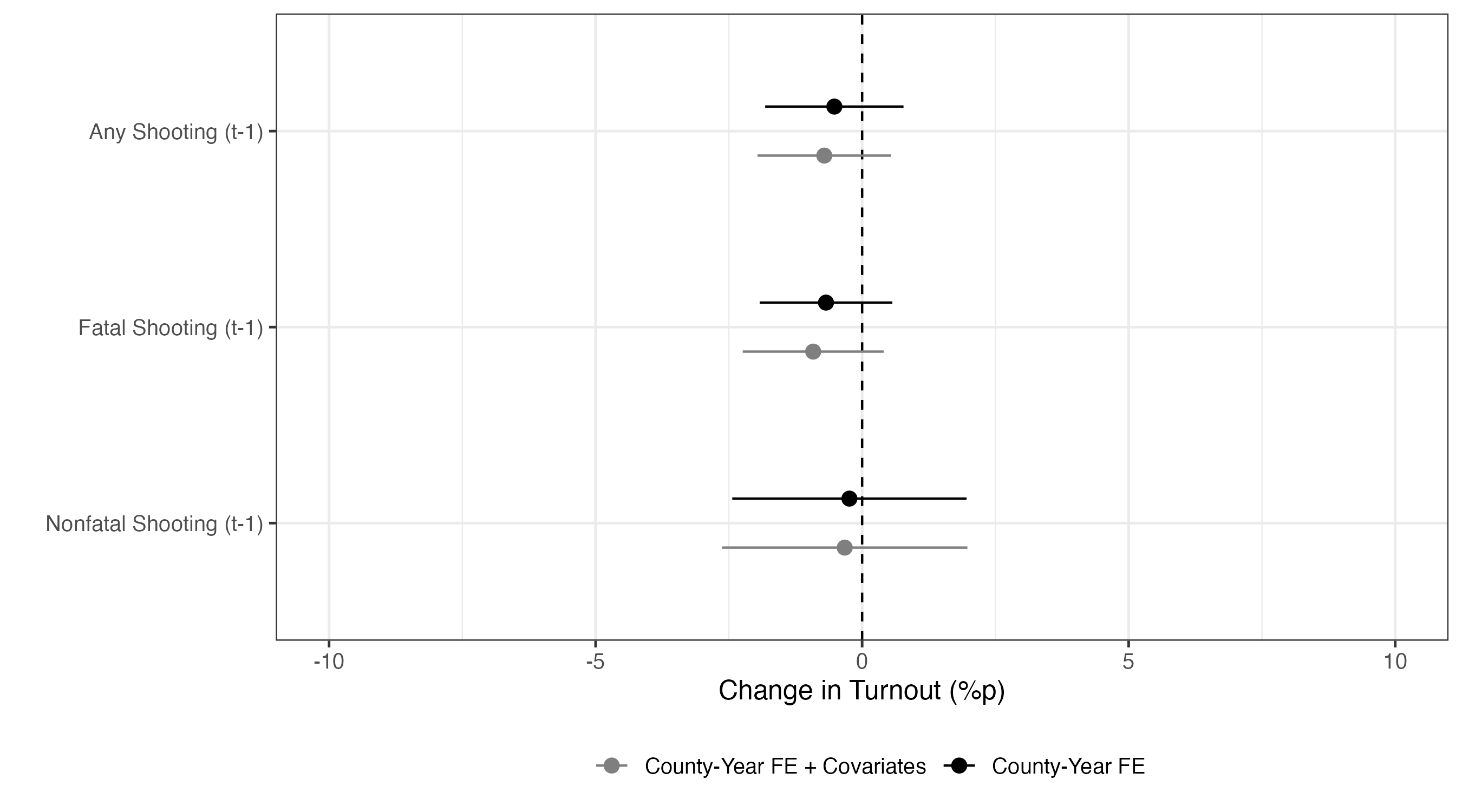
　いずれのモデルも統計的に有意な処置効果は確認されていない。これらの結果を表として報告するには紙がもったいない気もする。これらの結果はOnline Appendixに回し、本文中には処置効果の点推定値と95%信頼区間を示せば良いだろう。

　{broom}のtidy()関数で推定結果のみを抽出し、それぞれオブジェクトとして格納しておこう。

tidy_fit1 <- tidy(did_fit1, conf.int = TRUE)
tidy_fit2 <- tidy(did_fit2, conf.int = TRUE)
tidy_fit3 <- tidy(did_fit3, conf.int = TRUE)
tidy_fit4 <- tidy(did_fit4, conf.int = TRUE)
tidy_fit5 <- tidy(did_fit5, conf.int = TRUE)
tidy_fit6 <- tidy(did_fit6, conf.int = TRUE)

　全て確認する必要はないので、tidy_fit1のみを確認してみる。

tidy_fit1

      term   estimate std.error  statistic   p.value conf.low conf.high df
1 shooting -0.5210841 0.6456718 -0.8070417 0.4235426 -1.81861  0.776442 49
  outcome
1 turnout

　以上の6つの表形式オブジェクトを一つの表としてまとめる。それぞれのオブジェクトには共変量の有無_処置変数の種類の名前を付けよう。共変量なしのモデルはM1、ありのモデルはM2とする。処置変数はshootingの場合はTr1、fatal_shootingはTr2、non_fatal_shootingはTr3とする。

did_est1 <- bind_rows(list("M1_Tr1" = tidy_fit1,
                           "M2_Tr1" = tidy_fit2,
                           "M1_Tr2" = tidy_fit3,
                           "M2_Tr2" = tidy_fit4,
                           "M1_Tr3" = tidy_fit5,
                           "M2_Tr3" = tidy_fit6),
                      .id = "Model")

did_est1

    Model               term      estimate    std.error  statistic    p.value
1  M1_Tr1           shooting -5.210841e-01 6.456718e-01 -0.8070417 0.42354260
2  M2_Tr1           shooting -7.097922e-01 6.237320e-01 -1.1379763 0.26066411
3  M2_Tr1         population  8.028568e-06 5.688141e-06  1.4114574 0.16442833
4  M2_Tr1          non_white -3.483443e+01 1.557543e+01 -2.2364985 0.02990378
5  M2_Tr1   change_unem_rate  1.592020e-01 6.584450e-02  2.4178480 0.01937671
6  M1_Tr2     fatal_shooting -6.779229e-01 6.191749e-01 -1.0948810 0.27892152
7  M2_Tr2     fatal_shooting -9.179995e-01 6.576559e-01 -1.3958659 0.16904785
8  M2_Tr2         population  8.026778e-06 5.747531e-06  1.3965611 0.16883977
9  M2_Tr2          non_white -3.484436e+01 1.561829e+01 -2.2309975 0.03029042
10 M2_Tr2   change_unem_rate  1.591126e-01 6.591001e-02  2.4140886 0.01955574
11 M1_Tr3 non_fatal_shooting -2.387205e-01 1.093832e+00 -0.2182423 0.82814672
12 M2_Tr3 non_fatal_shooting -3.269742e-01 1.145303e+00 -0.2854915 0.77647098
13 M2_Tr3         population  7.821482e-06 5.712400e-06  1.3692110 0.17717684
14 M2_Tr3          non_white -3.481384e+01 1.561438e+01 -2.2296020 0.03038921
15 M2_Tr3   change_unem_rate  1.595359e-01 6.590170e-02  2.4208169 0.01923637
        conf.low     conf.high df outcome
1  -1.818610e+00  7.764420e-01 49 turnout
2  -1.963229e+00  5.436442e-01 49 turnout
3  -3.402178e-06  1.945932e-05 49 turnout
4  -6.613442e+01 -3.534428e+00 49 turnout
5   2.688251e-02  2.915215e-01 49 turnout
6  -1.922202e+00  5.663557e-01 49 turnout
7  -2.239609e+00  4.036096e-01 49 turnout
8  -3.523318e-06  1.957687e-05 49 turnout
9  -6.623047e+01 -3.458237e+00 49 turnout
10  2.666148e-02  2.915637e-01 49 turnout
11 -2.436859e+00  1.959418e+00 49 turnout
12 -2.628546e+00  1.974598e+00 49 turnout
13 -3.658017e-06  1.930098e-05 49 turnout
14 -6.619211e+01 -3.435580e+00 49 turnout
15  2.710152e-02  2.919704e-01 49 turnout

　続いて、処置効果のみを抽出する。処置効果はterm列の値が"shooting"、"fatal_shooting"、"non_fatal_shooting"のいずれかと一致する行であるため、filter()関数を使用する。

did_est1 <- did_est1 |>
  filter(term %in% c("shooting", "fatal_shooting", "non_fatal_shooting"))

did_est1

   Model               term   estimate std.error  statistic   p.value  conf.low
1 M1_Tr1           shooting -0.5210841 0.6456718 -0.8070417 0.4235426 -1.818610
2 M2_Tr1           shooting -0.7097922 0.6237320 -1.1379763 0.2606641 -1.963229
3 M1_Tr2     fatal_shooting -0.6779229 0.6191749 -1.0948810 0.2789215 -1.922202
4 M2_Tr2     fatal_shooting -0.9179995 0.6576559 -1.3958659 0.1690478 -2.239609
5 M1_Tr3 non_fatal_shooting -0.2387205 1.0938325 -0.2182423 0.8281467 -2.436859
6 M2_Tr3 non_fatal_shooting -0.3269742 1.1453027 -0.2854915 0.7764710 -2.628546
  conf.high df outcome
1 0.7764420 49 turnout
2 0.5436442 49 turnout
3 0.5663557 49 turnout
4 0.4036096 49 turnout
5 1.9594182 49 turnout
6 1.9745977 49 turnout

　ちなみにgrepl()関数を使うと、"shooting"が含まれる行を抽出することもできる。以下のコードは上記のコードと同じ機能をする。

did_est1 <- did_est1 |>
  filter(grepl("shooting", term))

　つづいて、Model列をModelとTreat列へ分割する。

did_est1 <- did_est1 |>
  separate(col  = Model,
           into = c("Model", "Treat"),
           sep  = "_")

did_est1

  Model Treat               term   estimate std.error  statistic   p.value
1    M1   Tr1           shooting -0.5210841 0.6456718 -0.8070417 0.4235426
2    M2   Tr1           shooting -0.7097922 0.6237320 -1.1379763 0.2606641
3    M1   Tr2     fatal_shooting -0.6779229 0.6191749 -1.0948810 0.2789215
4    M2   Tr2     fatal_shooting -0.9179995 0.6576559 -1.3958659 0.1690478
5    M1   Tr3 non_fatal_shooting -0.2387205 1.0938325 -0.2182423 0.8281467
6    M2   Tr3 non_fatal_shooting -0.3269742 1.1453027 -0.2854915 0.7764710
   conf.low conf.high df outcome
1 -1.818610 0.7764420 49 turnout
2 -1.963229 0.5436442 49 turnout
3 -1.922202 0.5663557 49 turnout
4 -2.239609 0.4036096 49 turnout
5 -2.436859 1.9594182 49 turnout
6 -2.628546 1.9745977 49 turnout

　可視化に入る前にModel列とTreat列の値を修正する。Model列の値が"M1"なら"County-Year FE"に、それ以外なら"County-Year FE + Covariates"とリコーディングする。戻り値が2種類だからif_else()を使う。Treat列の場合、戻り値が3つなので、recode()かcase_when()を使う。ここではrecode()を使ってリコーディングする。最後にModelとTreatを表示順番でfactor化し（fct_inorder()）、更に順番を逆転する（fct_rev()）。

did_est1 <- did_est1 |>
  mutate(Model = if_else(Model == "M1",
                           "County-Year FE", 
                           "County-Year FE + Covariates"),
         Treat = recode(Treat,
                        "Tr1" = "Any Shooting (t-1)",
                        "Tr2" = "Fatal Shooting (t-1)",
                        "Tr3" = "Nonfatal Shooting (t-1)"),
         Model = fct_rev(fct_inorder(Model)),
         Treat = fct_rev(fct_inorder(Treat)))

did_est1

                        Model                   Treat               term
1              County-Year FE      Any Shooting (t-1)           shooting
2 County-Year FE + Covariates      Any Shooting (t-1)           shooting
3              County-Year FE    Fatal Shooting (t-1)     fatal_shooting
4 County-Year FE + Covariates    Fatal Shooting (t-1)     fatal_shooting
5              County-Year FE Nonfatal Shooting (t-1) non_fatal_shooting
6 County-Year FE + Covariates Nonfatal Shooting (t-1) non_fatal_shooting
    estimate std.error  statistic   p.value  conf.low conf.high df outcome
1 -0.5210841 0.6456718 -0.8070417 0.4235426 -1.818610 0.7764420 49 turnout
2 -0.7097922 0.6237320 -1.1379763 0.2606641 -1.963229 0.5436442 49 turnout
3 -0.6779229 0.6191749 -1.0948810 0.2789215 -1.922202 0.5663557 49 turnout
4 -0.9179995 0.6576559 -1.3958659 0.1690478 -2.239609 0.4036096 49 turnout
5 -0.2387205 1.0938325 -0.2182423 0.8281467 -2.436859 1.9594182 49 turnout
6 -0.3269742 1.1453027 -0.2854915 0.7764710 -2.628546 1.9745977 49 turnout

　それでは{ggplot2}を使ってpoint-rangeプロットを作成してみよう。

did_est1 |>
  ggplot() +
  # x = 0の箇所に垂直線を引く。垂直線は破線（linetype = 2）とする。
  geom_vline(xintercept = 0, linetype = 2) +
  geom_pointrange(aes(x = estimate, xmin = conf.low, xmax = conf.high,
                      y = Treat, color = Model),
                  position = position_dodge2(1/2)) +
  labs(x = "Change in Turnout (%p)", y = "", color = "") +
  # 色を指定する。
  # Modelの値が County-Year FE なら黒、
  # County-Year FE + Covariates ならグレー、
  scale_color_manual(values = c("County-Year FE" = "black", 
                                "County-Year FE + Covariates" = "gray50")) +
  # 横軸の下限と上限を-10〜10とする。
  coord_cartesian(xlim = c(-10, 10)) +
  theme_bw(base_size = 12) +
  theme(legend.position = "bottom")

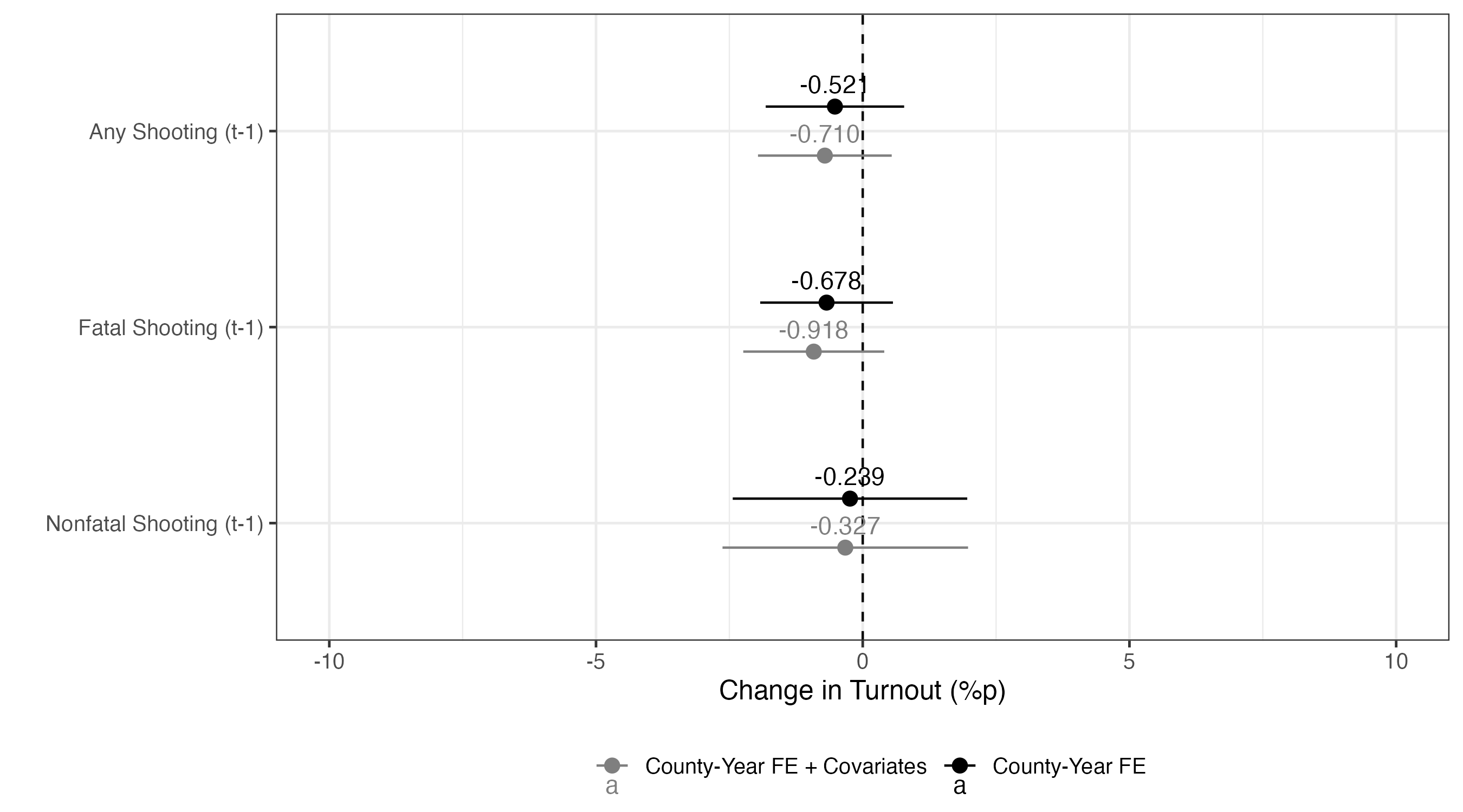
　元の論文を見ると、点の上に点推定値が書かれているが、私たちもこれを真似してみよう。文字列をプロットするレイヤーはgeom_text()とgeom_label()、annotate()があるが、ここではgeom_text()を使用する。文字列が表示される横軸上の位置（x）と縦軸上の位置（y）、そして出力する文字列（label）をマッピングする。点推定値は3桁まで出力したいので、sprintf()を使って、3桁に丸める。ただし、これだけだと点と文字が重なってしまう。vjustを-0.75にすることで、出力する文字列を点の位置を上の方向へ若干ずらすことができる。

did_est1 |>
  ggplot() +
  geom_vline(xintercept = 0, linetype = 2) +
  geom_pointrange(aes(x = estimate, xmin = conf.low, xmax = conf.high,
                      y = Treat, color = Model),
                  position = position_dodge2(1/2)) +
  geom_text(aes(x = estimate, y = Treat, color = Model, 
                label = sprintf("%.3f", estimate)),
            position = position_dodge2(1/2),
            vjust = -0.75) +
  labs(x = "Change in Turnout (%p)", y = "", color = "") +
  scale_color_manual(values = c("County-Year FE" = "black", 
                                "County-Year FE + Covariates" = "gray50")) +
  coord_cartesian(xlim = c(-10, 10)) +
  theme_bw(base_size = 12) +
  theme(legend.position = "bottom")

　ちなみにこのコードを見ると、geom_pointrange()とgeom_text()はx、y、colorを共有しているので、ggplot()内でマッピングすることもできる。

did_est1 |>
  ggplot(aes(x = estimate, y = Treat, color = Model)) +
  geom_vline(xintercept = 0, linetype = 2) +
  geom_pointrange(aes(xmin = conf.low, xmax = conf.high),
                  position = position_dodge2(1/2)) +
  geom_text(aes(label = sprintf("%.3f", estimate)),
            position = position_dodge2(1/2),
            vjust = -0.75) +
  labs(x = "Change in Turnout (%p)", y = "", color = "") +
  scale_color_manual(values = c("County-Year FE" = "black", 
                                "County-Year FE + Covariates" = "gray50")) +
  coord_cartesian(xlim = c(-10, 10)) +
  theme_bw(base_size = 12) +
  theme(legend.position = "bottom")

　続いて、民主党候補者の得票率（demvote）を応答変数として6つのモデルを推定し、同じ作業を繰り返す。

did_fit7 <- lm_robust(demvote ~ shooting, 
                      data          = did_df, 
                      fixed_effects = ~year_f + county_f,
                      clusters      = state_f,
                      se_type       = "stata")

did_fit8 <- lm_robust(demvote ~ shooting + 
                        population + non_white + change_unem_rate, 
                      data          = did_df, 
                      fixed_effects = ~year_f + county_f,
                      clusters      = state_f,
                      se_type       = "stata")

did_fit9 <- lm_robust(demvote ~ fatal_shooting, 
                      data          = did_df, 
                      fixed_effects = ~year_f + county_f,
                      clusters      = state_f,
                      se_type       = "stata")

did_fit10 <- lm_robust(demvote ~ fatal_shooting + 
                         population + non_white + change_unem_rate, 
                       data          = did_df, 
                       fixed_effects = ~year_f + county_f,
                       clusters      = state_f,
                       se_type       = "stata")

did_fit11 <- lm_robust(demvote ~ non_fatal_shooting, 
                       data          = did_df, 
                       fixed_effects = ~year_f + county_f,
                       clusters      = state_f,
                       se_type       = "stata")

did_fit12 <- lm_robust(demvote ~ non_fatal_shooting + 
                         population + non_white + change_unem_rate, 
                       data          = did_df, 
                       fixed_effects = ~year_f + county_f,
                       clusters      = state_f,
                       se_type       = "stata")

modelsummary(list("Model 7"  = did_fit7,  "Model 8"  = did_fit8, 
                  "Model 9"  = did_fit9,  "Model 10" = did_fit10, 
                  "Model 11" = did_fit11, "Model 12" = did_fit12))

	Model 7	Model 8	Model 9	Model 10	Model 11	Model 12
shooting	4.513	2.364
	(0.875)	(0.737)
population		0.000		0.000		0.000
		(0.000)		(0.000)		(0.000)
non_white		86.873		86.866		86.796
		(17.863)		(17.855)		(17.855)
change_unem_rate		−0.139		−0.139		−0.140
		(0.127)		(0.128)		(0.127)
fatal_shooting			4.404	1.782
			(1.092)	(0.836)
non_fatal_shooting					4.217	2.930
					(1.298)	(1.037)
Num.Obs.	18627	18627	18627	18627	18627	18627
R2	0.882	0.894	0.882	0.894	0.882	0.894
R2 Adj.	0.859	0.873	0.859	0.873	0.859	0.873
AIC	110745.2	108755.4	110772.0	108768.2	110786.5	108762.1
BIC	110760.8	108794.6	110787.7	108807.3	110802.2	108801.3
RMSE	4.73	4.48	4.73	4.48	4.73	4.48
Std.Errors	by: state_f	by: state_f	by: state_f	by: state_f	by: state_f	by: state_f

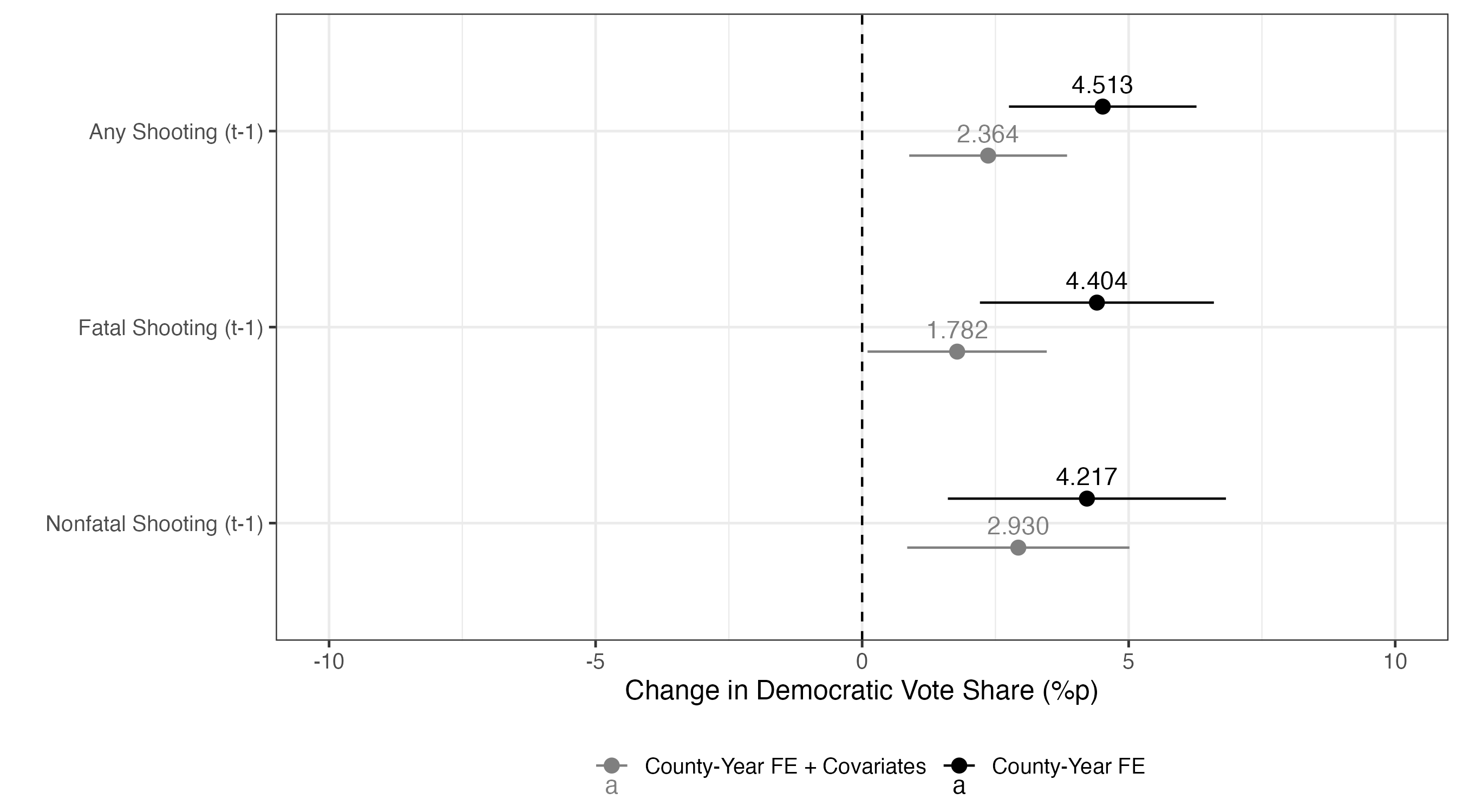
　今回はいずれも統計的に有意な結果が得られている。例えば、モデル7（did_fit7）の場合、処置効果の推定値は4.513である。これは学校内銃撃事件が発生したカウンティーの場合、大統領選挙において民主党候補者の得票率が約4.513%p増加することを意味する。

　以上の結果を図としてまとめてみよう。

tidy_fit7  <- tidy(did_fit7)
tidy_fit8  <- tidy(did_fit8)
tidy_fit9  <- tidy(did_fit9)
tidy_fit10 <- tidy(did_fit10)
tidy_fit11 <- tidy(did_fit11)
tidy_fit12 <- tidy(did_fit12)

did_est2 <- bind_rows(list("M1_Tr1" = tidy_fit7,
                           "M2_Tr1" = tidy_fit8,
                           "M1_Tr2" = tidy_fit9,
                           "M2_Tr2" = tidy_fit10,
                           "M1_Tr3" = tidy_fit11,
                           "M2_Tr3" = tidy_fit12),
                      .id = "Model")

did_est2

    Model               term      estimate    std.error statistic      p.value
1  M1_Tr1           shooting  4.513237e+00 8.752702e-01  5.156393 4.514820e-06
2  M2_Tr1           shooting  2.363839e+00 7.367346e-01  3.208536 2.353748e-03
3  M2_Tr1         population  3.174252e-05 6.778757e-06  4.682646 2.275534e-05
4  M2_Tr1          non_white  8.687344e+01 1.786287e+01  4.863352 1.234074e-05
5  M2_Tr1   change_unem_rate -1.389392e-01 1.274198e-01 -1.090405 2.808682e-01
6  M1_Tr2     fatal_shooting  4.404109e+00 1.091944e+00  4.033274 1.920110e-04
7  M2_Tr2     fatal_shooting  1.782393e+00 8.363792e-01  2.131083 3.812471e-02
8  M2_Tr2         population  3.206812e-05 6.801197e-06  4.715070 2.039958e-05
9  M2_Tr2          non_white  8.686629e+01 1.785535e+01  4.865000 1.227169e-05
10 M2_Tr2   change_unem_rate -1.392341e-01 1.275138e-01 -1.091914 2.802109e-01
11 M1_Tr3 non_fatal_shooting  4.216683e+00 1.298056e+00  3.248460 2.098382e-03
12 M2_Tr3 non_fatal_shooting  2.929866e+00 1.037217e+00  2.824737 6.825655e-03
13 M2_Tr3         population  3.229215e-05 6.717999e-06  4.806810 1.495567e-05
14 M2_Tr3          non_white  8.679618e+01 1.785514e+01  4.861131 1.243440e-05
15 M2_Tr3   change_unem_rate -1.400321e-01 1.274994e-01 -1.098296 2.774427e-01
        conf.low    conf.high df outcome
1   2.754316e+00 6.272159e+00 49 demvote
2   8.833157e-01 3.844363e+00 49 demvote
3   1.812010e-05 4.536494e-05 49 demvote
4   5.097665e+01 1.227702e+02 49 demvote
5  -3.949989e-01 1.171206e-01 49 demvote
6   2.209766e+00 6.598453e+00 49 demvote
7   1.016261e-01 3.463160e+00 49 demvote
8   1.840061e-05 4.573564e-05 49 demvote
9   5.098461e+01 1.227480e+02 49 demvote
10 -3.954828e-01 1.170146e-01 49 demvote
11  1.608142e+00 6.825225e+00 49 demvote
12  8.454996e-01 5.014232e+00 49 demvote
13  1.879182e-05 4.579247e-05 49 demvote
14  5.091493e+01 1.226774e+02 49 demvote
15 -3.962518e-01 1.161876e-01 49 demvote

did_est2 <- did_est2 |>
  filter(grepl("shooting", term))

did_est2

   Model               term estimate std.error statistic      p.value  conf.low
1 M1_Tr1           shooting 4.513237 0.8752702  5.156393 4.514820e-06 2.7543158
2 M2_Tr1           shooting 2.363839 0.7367346  3.208536 2.353748e-03 0.8833157
3 M1_Tr2     fatal_shooting 4.404109 1.0919440  4.033274 1.920110e-04 2.2097656
4 M2_Tr2     fatal_shooting 1.782393 0.8363792  2.131083 3.812471e-02 0.1016261
5 M1_Tr3 non_fatal_shooting 4.216683 1.2980560  3.248460 2.098382e-03 1.6081422
6 M2_Tr3 non_fatal_shooting 2.929866 1.0372173  2.824737 6.825655e-03 0.8454996
  conf.high df outcome
1  6.272159 49 demvote
2  3.844363 49 demvote
3  6.598453 49 demvote
4  3.463160 49 demvote
5  6.825225 49 demvote
6  5.014232 49 demvote

did_est2 <- did_est2 |>
  separate(col  = Model,
           into = c("Model", "Treat"),
           sep  = "_")

did_est2

  Model Treat               term estimate std.error statistic      p.value
1    M1   Tr1           shooting 4.513237 0.8752702  5.156393 4.514820e-06
2    M2   Tr1           shooting 2.363839 0.7367346  3.208536 2.353748e-03
3    M1   Tr2     fatal_shooting 4.404109 1.0919440  4.033274 1.920110e-04
4    M2   Tr2     fatal_shooting 1.782393 0.8363792  2.131083 3.812471e-02
5    M1   Tr3 non_fatal_shooting 4.216683 1.2980560  3.248460 2.098382e-03
6    M2   Tr3 non_fatal_shooting 2.929866 1.0372173  2.824737 6.825655e-03
   conf.low conf.high df outcome
1 2.7543158  6.272159 49 demvote
2 0.8833157  3.844363 49 demvote
3 2.2097656  6.598453 49 demvote
4 0.1016261  3.463160 49 demvote
5 1.6081422  6.825225 49 demvote
6 0.8454996  5.014232 49 demvote

did_est2 <- did_est2 |>
  mutate(Model = if_else(Model == "M1",
                           "County-Year FE", 
                           "County-Year FE + Covariates"),
         Treat = recode(Treat,
                        "Tr1" = "Any Shooting (t-1)",
                        "Tr2" = "Fatal Shooting (t-1)",
                        "Tr3" = "Nonfatal Shooting (t-1)"),
         Model = fct_rev(fct_inorder(Model)),
         Treat = fct_rev(fct_inorder(Treat)))

did_est2

                        Model                   Treat               term
1              County-Year FE      Any Shooting (t-1)           shooting
2 County-Year FE + Covariates      Any Shooting (t-1)           shooting
3              County-Year FE    Fatal Shooting (t-1)     fatal_shooting
4 County-Year FE + Covariates    Fatal Shooting (t-1)     fatal_shooting
5              County-Year FE Nonfatal Shooting (t-1) non_fatal_shooting
6 County-Year FE + Covariates Nonfatal Shooting (t-1) non_fatal_shooting
  estimate std.error statistic      p.value  conf.low conf.high df outcome
1 4.513237 0.8752702  5.156393 4.514820e-06 2.7543158  6.272159 49 demvote
2 2.363839 0.7367346  3.208536 2.353748e-03 0.8833157  3.844363 49 demvote
3 4.404109 1.0919440  4.033274 1.920110e-04 2.2097656  6.598453 49 demvote
4 1.782393 0.8363792  2.131083 3.812471e-02 0.1016261  3.463160 49 demvote
5 4.216683 1.2980560  3.248460 2.098382e-03 1.6081422  6.825225 49 demvote
6 2.929866 1.0372173  2.824737 6.825655e-03 0.8454996  5.014232 49 demvote

did_est2 |>
  ggplot() +
  geom_vline(xintercept = 0, linetype = 2) +
  geom_pointrange(aes(x = estimate, xmin = conf.low, xmax = conf.high,
                      y = Treat, color = Model),
                  position = position_dodge2(1/2)) +
  geom_text(aes(x = estimate, y = Treat, color = Model, 
                label = sprintf("%.3f", estimate)),
            position = position_dodge2(1/2),
            vjust = -0.75) +
  labs(x = "Change in Democratic Vote Share (%p)", y = "", color = "") +
  scale_color_manual(values = c("County-Year FE" = "black", 
                                "County-Year FE + Covariates" = "gray50")) +
  coord_cartesian(xlim = c(-10, 10)) +
  theme_bw(base_size = 12) +
  theme(legend.position = "bottom")

　最後に、これまで作成した2つの図を一つにまとめてみよう。bind_rows()関数を使い、それぞれの表に識別子（Outcome）を与える。

did_est <- bind_rows(list("Out1" = did_est1,
                          "Out2" = did_est2),
                     .id = "Outcome")

did_est

   Outcome                       Model                   Treat
1     Out1              County-Year FE      Any Shooting (t-1)
2     Out1 County-Year FE + Covariates      Any Shooting (t-1)
3     Out1              County-Year FE    Fatal Shooting (t-1)
4     Out1 County-Year FE + Covariates    Fatal Shooting (t-1)
5     Out1              County-Year FE Nonfatal Shooting (t-1)
6     Out1 County-Year FE + Covariates Nonfatal Shooting (t-1)
7     Out2              County-Year FE      Any Shooting (t-1)
8     Out2 County-Year FE + Covariates      Any Shooting (t-1)
9     Out2              County-Year FE    Fatal Shooting (t-1)
10    Out2 County-Year FE + Covariates    Fatal Shooting (t-1)
11    Out2              County-Year FE Nonfatal Shooting (t-1)
12    Out2 County-Year FE + Covariates Nonfatal Shooting (t-1)
                 term   estimate std.error  statistic      p.value   conf.low
1            shooting -0.5210841 0.6456718 -0.8070417 4.235426e-01 -1.8186103
2            shooting -0.7097922 0.6237320 -1.1379763 2.606641e-01 -1.9632286
3      fatal_shooting -0.6779229 0.6191749 -1.0948810 2.789215e-01 -1.9222015
4      fatal_shooting -0.9179995 0.6576559 -1.3958659 1.690478e-01 -2.2396086
5  non_fatal_shooting -0.2387205 1.0938325 -0.2182423 8.281467e-01 -2.4368592
6  non_fatal_shooting -0.3269742 1.1453027 -0.2854915 7.764710e-01 -2.6285461
7            shooting  4.5132372 0.8752702  5.1563930 4.514820e-06  2.7543158
8            shooting  2.3638394 0.7367346  3.2085357 2.353748e-03  0.8833157
9      fatal_shooting  4.4041092 1.0919440  4.0332738 1.920110e-04  2.2097656
10     fatal_shooting  1.7823931 0.8363792  2.1310825 3.812471e-02  0.1016261
11 non_fatal_shooting  4.2166835 1.2980560  3.2484602 2.098382e-03  1.6081422
12 non_fatal_shooting  2.9298657 1.0372173  2.8247368 6.825655e-03  0.8454996
   conf.high df outcome
1  0.7764420 49 turnout
2  0.5436442 49 turnout
3  0.5663557 49 turnout
4  0.4036096 49 turnout
5  1.9594182 49 turnout
6  1.9745977 49 turnout
7  6.2721585 49 demvote
8  3.8443631 49 demvote
9  6.5984529 49 demvote
10 3.4631600 49 demvote
11 6.8252248 49 demvote
12 5.0142319 49 demvote

　Outcome列のリコーディングし、factor化する。

did_est <- did_est |>
  mutate(Outcome = if_else(Outcome == "Out1",
                           "Change in Turnout (%p)",
                           "Change in Democratic Vote Share (%p)"),
         Outcome = fct_inorder(Outcome))

did_est

                                Outcome                       Model
1                Change in Turnout (%p)              County-Year FE
2                Change in Turnout (%p) County-Year FE + Covariates
3                Change in Turnout (%p)              County-Year FE
4                Change in Turnout (%p) County-Year FE + Covariates
5                Change in Turnout (%p)              County-Year FE
6                Change in Turnout (%p) County-Year FE + Covariates
7  Change in Democratic Vote Share (%p)              County-Year FE
8  Change in Democratic Vote Share (%p) County-Year FE + Covariates
9  Change in Democratic Vote Share (%p)              County-Year FE
10 Change in Democratic Vote Share (%p) County-Year FE + Covariates
11 Change in Democratic Vote Share (%p)              County-Year FE
12 Change in Democratic Vote Share (%p) County-Year FE + Covariates
                     Treat               term   estimate std.error  statistic
1       Any Shooting (t-1)           shooting -0.5210841 0.6456718 -0.8070417
2       Any Shooting (t-1)           shooting -0.7097922 0.6237320 -1.1379763
3     Fatal Shooting (t-1)     fatal_shooting -0.6779229 0.6191749 -1.0948810
4     Fatal Shooting (t-1)     fatal_shooting -0.9179995 0.6576559 -1.3958659
5  Nonfatal Shooting (t-1) non_fatal_shooting -0.2387205 1.0938325 -0.2182423
6  Nonfatal Shooting (t-1) non_fatal_shooting -0.3269742 1.1453027 -0.2854915
7       Any Shooting (t-1)           shooting  4.5132372 0.8752702  5.1563930
8       Any Shooting (t-1)           shooting  2.3638394 0.7367346  3.2085357
9     Fatal Shooting (t-1)     fatal_shooting  4.4041092 1.0919440  4.0332738
10    Fatal Shooting (t-1)     fatal_shooting  1.7823931 0.8363792  2.1310825
11 Nonfatal Shooting (t-1) non_fatal_shooting  4.2166835 1.2980560  3.2484602
12 Nonfatal Shooting (t-1) non_fatal_shooting  2.9298657 1.0372173  2.8247368
        p.value   conf.low conf.high df outcome
1  4.235426e-01 -1.8186103 0.7764420 49 turnout
2  2.606641e-01 -1.9632286 0.5436442 49 turnout
3  2.789215e-01 -1.9222015 0.5663557 49 turnout
4  1.690478e-01 -2.2396086 0.4036096 49 turnout
5  8.281467e-01 -2.4368592 1.9594182 49 turnout
6  7.764710e-01 -2.6285461 1.9745977 49 turnout
7  4.514820e-06  2.7543158 6.2721585 49 demvote
8  2.353748e-03  0.8833157 3.8443631 49 demvote
9  1.920110e-04  2.2097656 6.5984529 49 demvote
10 3.812471e-02  0.1016261 3.4631600 49 demvote
11 2.098382e-03  1.6081422 6.8252248 49 demvote
12 6.825655e-03  0.8454996 5.0142319 49 demvote

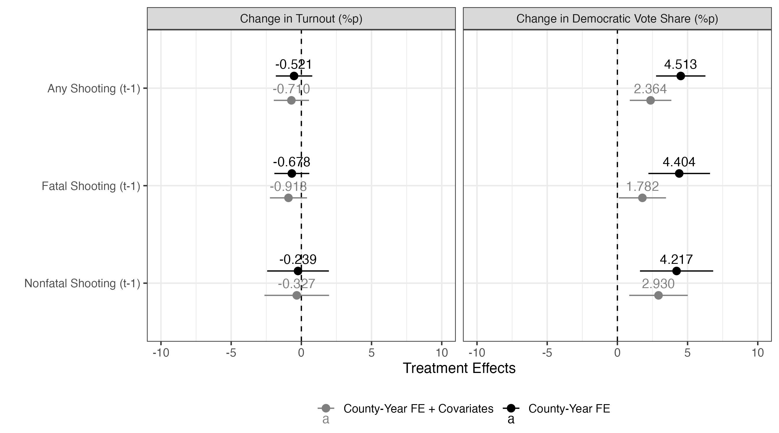
　図の作り方はこれまでと変わらないが、ファセット分割を行うため、facet_wrap()レイヤーを追加する。

did_est |>
  ggplot() +
  geom_vline(xintercept = 0, linetype = 2) +
  geom_pointrange(aes(x = estimate, xmin = conf.low, xmax = conf.high,
                      y = Treat, color = Model),
                  position = position_dodge2(1/2)) +
  geom_text(aes(x = estimate, y = Treat, color = Model, 
                label = sprintf("%.3f", estimate)),
            position = position_dodge2(1/2),
            vjust = -0.75) +
  labs(x = "Treatment Effects", y = "", color = "") +
  scale_color_manual(values = c("County-Year FE" = "black", 
                                "County-Year FE + Covariates" = "gray50")) +
  coord_cartesian(xlim = c(-10, 10)) +
  facet_wrap(~Outcome, ncol = 2) +
  theme_bw(base_size = 12) +
  theme(legend.position = "bottom")

　以上の結果から「学校内銃撃事件の発生は投票参加を促すとは言えないものの、民主党候補者の得票率を上げる」ということが言えよう。

SCM

　ここでは、差分の差分法の応用としてSynthetic Control Method（SCM）を{gsynth}パッケージの使い方に重点を起きながら説明する。Synthetic Control MethodをRに実装したパッケージは{Synth}、{gsynth}、{bpCausal}などがある。SCMの代表的な論文の一つであるAbadie et al.（2015）は{Synth}パッケージを使っているが、使い方はかなり複雑である。したがって、ここでは使い方が最も簡単な{gsynth}パッケージについて説明する²。

　ここで使用するのは歴代参院選（第7回以降）における都道府県の投票率である³。処置変数は第24回参院選から導入された「合区」だ。具体的には鳥取選挙区と島根選挙区が「鳥取・島根選挙区」に、徳島選挙区と高知選挙区が「徳島・高知選挙区」として合区されたか否かである。合区によって自分の1票の価値がほぼ半分に下がり、投票参加を妨げたのではないかという議論もあるが、本当だろうか。

scm_df <- read_csv("data/did_data5.csv")

scm_df

# A tibble: 938 × 9
   Election PrefCode PrefName_E PrefName_J Eligible  Voters EffVote Magnitude
      <dbl>    <dbl> <chr>      <chr>         <dbl>   <dbl>   <dbl>     <dbl>
 1        7        1 Hokkaido   北海道      2903802 1829347 1683764         4
 2        7        2 Aomori     青森県       823336  509254  478380         1
 3        7        3 Iwate      岩手県       849109  619767  591977         1
 4        7        4 Miyagi     宮城県      1049109  694827  666205         1
 5        7        5 Akita      秋田県       771983  591315  558603         1
 6        7        6 Yamagata   山形県       784438  636550  615414         1
 7        7        7 Fukushima  福島県      1123975  893381  855609         2
 8        7        8 Ibaraki    茨城県      1246254  785174  750181         2
 9        7        9 Tochigi    栃木県       909245  638413  614249         2
10        7       10 Gunma      群馬県       990083  719678  690448         2
# ℹ 928 more rows
# ℹ 1 more variable: Candidates <dbl>

scm_df |>
  select(Eligible:Candidates) |>
  descr(stats = c("mean", "sd", "min", "max", "n.valid"),
        transpose = TRUE, order = "p")

Descriptive Statistics  

                         Mean      Std.Dev         Min           Max   N.Valid
---------------- ------------ ------------ ----------- ------------- ---------
        Eligible   1933435.87   1867850.63   364184.00   11454822.00    938.00
          Voters   1139531.46   1029039.25   226580.00    6477709.00    938.00
         EffVote   1096934.10    997876.11   217637.00    6298466.00    938.00
       Magnitude         1.60         0.87        1.00          6.00    938.00
      Candidates         5.49         5.42        2.00         72.00    938.00

変数名	説明	備考
`Election`	選挙	第XX回参議院議員通常選挙
`PrefCode`	都道府県	JIS規格コード
`PrefName_E`	都道府県	英語
`PrefName_J`	都道府県	日本語
`Eligible`	有権者数
`Voters`	投票者数
`EffVote`	有効投票数
`Magnitude`	定数
`Candidates`	候補者数

　合区された選挙区における定数および候補者数の扱いについてだが、たとえば島根選挙区の場合、合区前の定数は1である。合区後の鳥取・島根選挙区も定数1だ。この場合、合区後の島根「県」の定数を1にするか0.5にするか、そして候補者数も合区における候補者数にすべきか、2に割るかが問題となるが、ここでは定数を1とし、候補者数も合区における候補者数とした。このようなコーディングが実証上、正しいかどうかは分からないが、実習の段階では問題ないだろう。

　それでは、データを以下のように加工する。

Treatという変数を作成する。PrefNameが「鳥取県」、「島根県」、「徳島県」、「高知県」であり、Electionが24以上なら1、それ以外のケースは0とする。
Turnoutという変数を作成する。投票者数（Voters）を有権者数（Eligible）で割り、100を掛ける。
Spoiltという変数を作成する。有効投票数（EffVote）を有権者数（Eligible）で割った値を1から引き、100を掛ける。
都道府県名（PrefName_E）をfactor変数に変換し、PrefName_Fという列として追加します。水準（levels）の順番はデータの出現順とする。
都道府県名（PrefName_J）をfactor化し、要素の順番はscm_df内における表示順番とする。

scm_df <- scm_df |>
  mutate(Treat      = if_else(PrefName_E %in% c("Tottori", "Shimane",
                                                "Tokushima","Kochi") &
                                Election >= 24, 1, 0),
         Turnout    = Voters / Eligible * 100,
         Spoilt     = (1 - (EffVote / Voters)) * 100,
         PrefName_J = fct_inorder(PrefName_J))

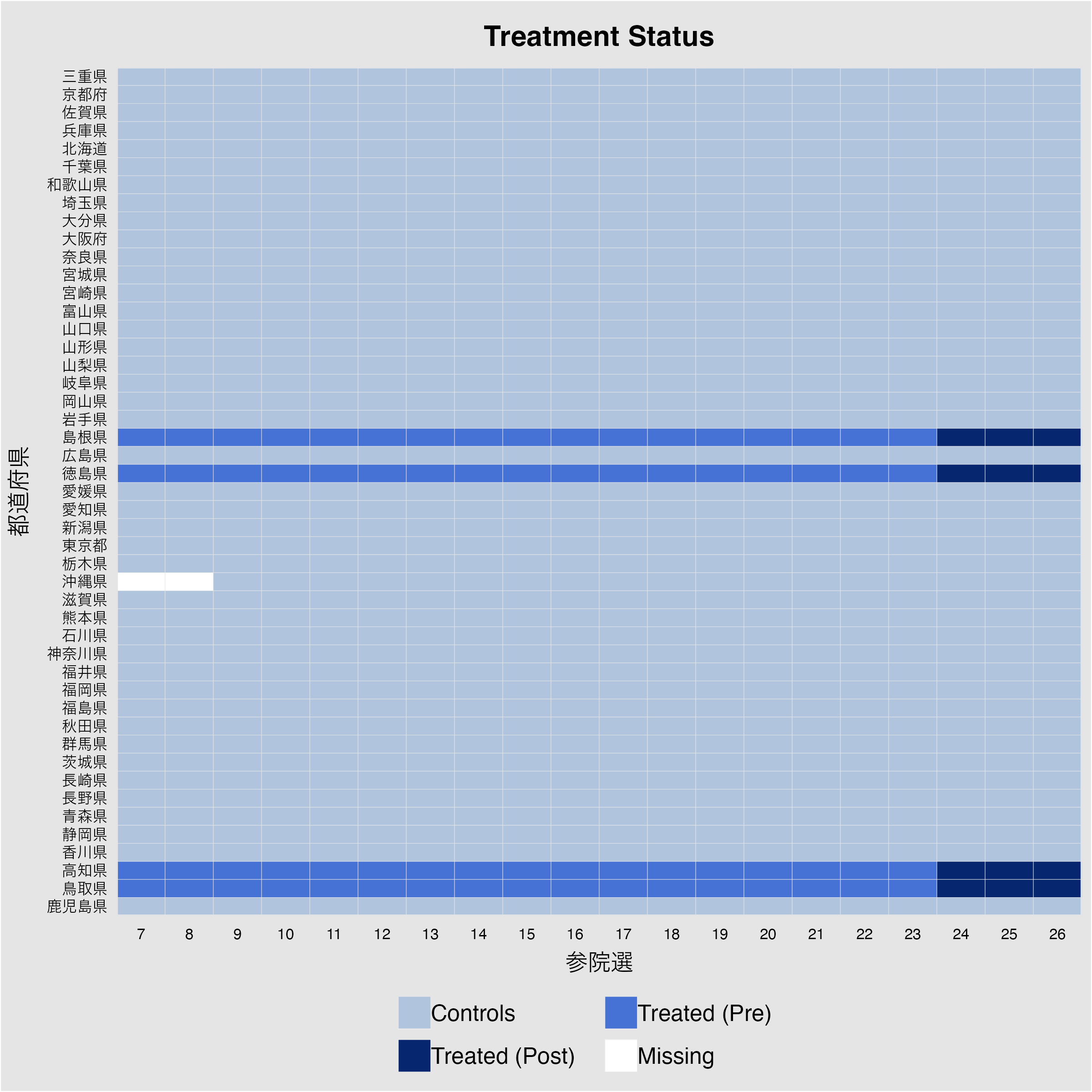
　本格的な分析に入る前に、各ケースの処置有無を可視化してみよう。パネルデータの確認には{panelView}パッケージのpanelview()関数を使う。第一引数は応答変数 ~ 処置変数であり、data引数にデータフレームのオブジェクト名を指定する。また、indexにはユニットと時間を表す変数名を長さ2のcharacter型ベクトルとして指定します。ここでは"PrefName_J"と"Election"である。最後に、pre.post = TRUEを指定すると、処置前後を色分けしてくれるので、見やすくなる。

panelview(Turnout ~ Treat, data = scm_df, 
          index = c("PrefName_J", "Election"), pre.post = TRUE,
          xlab = "参院選", ylab = "都道府県")

　これを見ると処置を受けるケースが4県であり、どれも第24回参院選から処置を受けることが分かる。また、沖縄県の場合、第7・8回参院選のデータが欠損していることが分かる。

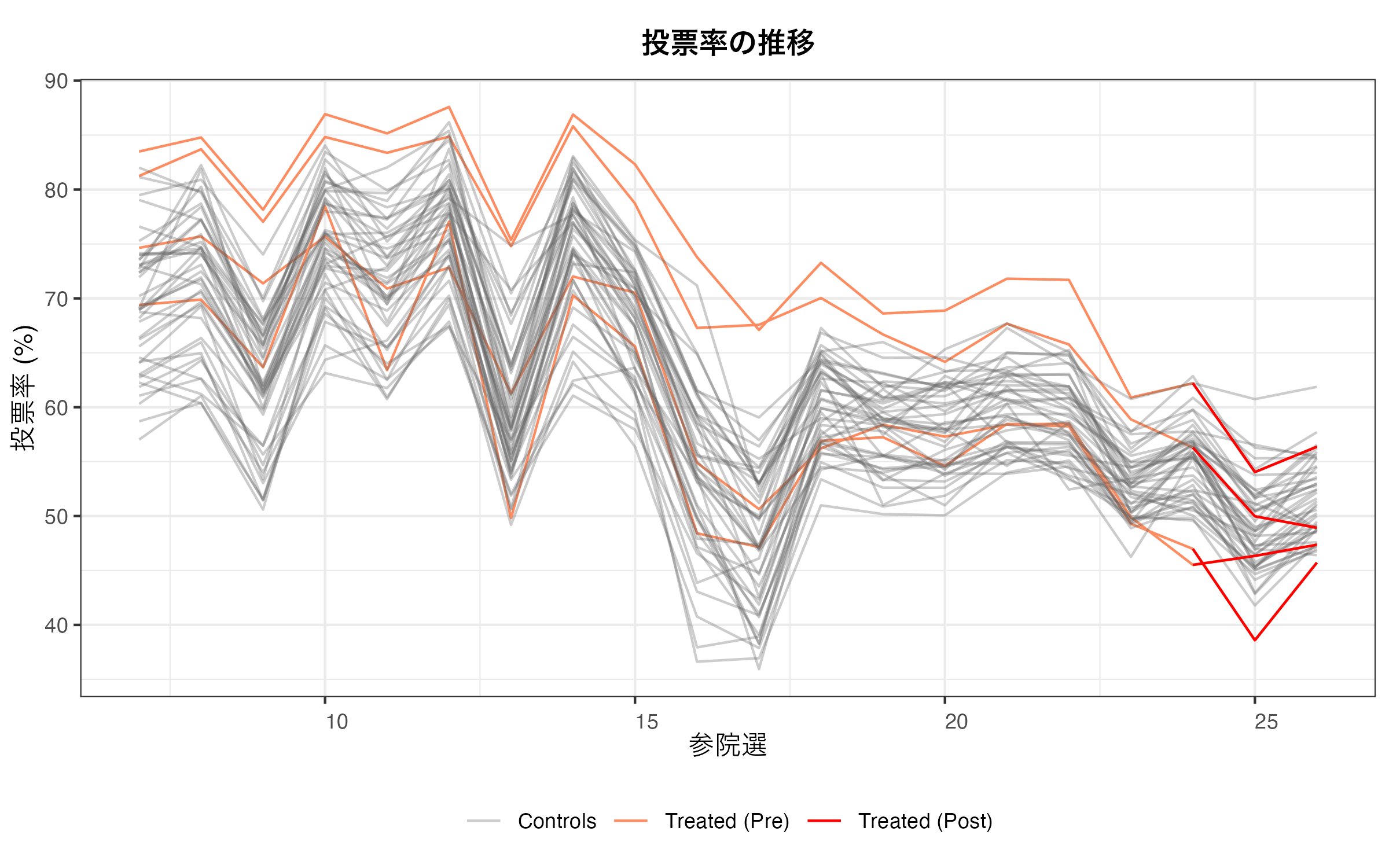
　次は投票率の変化を時系列的に示してみよう。使い方は先ほどとほぼ同じだが、panelView()内にtype = "outcome"引数を追加する。

panelview(Turnout ~ Treat, data = scm_df, 
          index = c("PrefName_J", "Election"), 
          type  = "outcome",
          main  = "投票率の推移",
          xlab  = "参院選",
          ylab  = "投票率 (%)")

　これを見ると、都道府県内における投票率の変化にはバラツキがあるが、傾向としてはかなり似通っていることが分かる。また、処置後の変化（濃い青の線）を見ると、他の都道府県よりかなり落ちているようにも見える。これは合区によって何かの変化が生じた可能性があることを示唆している。

　それではSCMをやってみよう。基本的な使い方はlm()関数に近いが、それでも必要な引数がそれなりにある。ここではその一部を紹介する。

第1引数は応答変数 ~ 処置変数 + 統制変数1 + 統制変数2 + ...であり、統制変数は必須ではない。ここでは統制変数として定数（Magnitude）と候補者数（Candidates）を使用する。
dataにはデータフレームのオブジェクト名を指定する。
indexはpanelview()と同じだが、一つ注意が必要です。それは、ユニットを表す変数をこれまではfactor化された"PrefName_J"を使ってきたが、factor化されていない"PrefName_E"にすることだ。まだ開発途上のパッケージということもあり、ユニット変数がfactor型だと、正しく推定できない。PrefName_Eはfactor型でなくcharacter型ですので、問題ない（あえてPrefName_Eをfactor化しなかったのはこのためである）。また、numeric型であるPrefCodeを指定すれば良い。。
forceは固定効果をユニットレベルにするか、時間レベルにするか、両方にするか、あるいはなしにするかを意味する。既定値はユニットレベル（"unit"）だが、ここでは両方（"two-way"）にする。
seは標準誤差を計算するか否かであり、既定値はFALSEである。ここでは標準誤差も計算するためにTRUEに指定する。標準誤差を計算しない場合、計算が早く終わる。
inferenceは推定方法を意味し、既定値はノンパラメトリック推定（"nonparametric"）です。ただし、処置ケースが少ない場合、パラメトリック推定が推奨されているため、ここでは"parametric"を指定する。
nbootsは標準誤差を計算する際に使用されるブートストラッピングの回数である。既定値は200ですが、ここでは500回にする。
parallelは並列計算の有無を意味する。既定値はTRUEで、このままでも通常は問題ない。ただし、R Markdown上で{gsynth}を使用する場合は並列計算ができないため、FALSEにしておく（処理時間が倍以上になる）。

scm_fit <- gsynth(Turnout ~ Treat + Magnitude + Candidates, 
                  data = scm_df, index = c("PrefName_E", "Election"), 
                  force = "two-way", se = TRUE, inference = "parametric",
                  nboots = 500, parallel = TRUE)

print(scm_fit)

Call:
gsynth.formula(formula = Turnout ~ Treat + Magnitude + Candidates, 
    data = scm_df, index = c("PrefName_E", "Election"), force = "two-way", 
    se = TRUE, nboots = 500, inference = "parametric", parallel = FALSE)

Average Treatment Effect on the Treated:
        Estimate  S.E. CI.lower CI.upper   p.value
ATT.avg   -6.563 1.453   -9.411   -3.715 6.285e-06

   ~ by Period (including Pre-treatment Periods):
         ATT   S.E.  CI.lower CI.upper   p.value n.Treated
-16  0.09054 1.1863  -2.23456   2.4156 9.392e-01         0
-15 -0.56609 1.2318  -2.98034   1.8482 6.458e-01         0
-14  3.32790 1.0729   1.22507   5.4307 1.923e-03         0
-13  1.44804 1.0538  -0.61729   3.5134 1.694e-01         0
-12 -1.53058 1.0050  -3.50026   0.4391 1.278e-01         0
-11 -1.21442 0.8881  -2.95504   0.5262 1.715e-01         0
-10 -2.51664 1.1633  -4.79674  -0.2365 3.052e-02         0
-9  -1.69683 1.1052  -3.86290   0.4692 1.247e-01         0
-8   1.12683 1.0510  -0.93313   3.1868 2.837e-01         0
-7  -1.03078 1.1934  -3.36985   1.3083 3.877e-01         0
-6   3.60723 1.6353   0.40204   6.8124 2.740e-02         0
-5  -0.85728 1.1320  -3.07604   1.3615 4.489e-01         0
-4   0.34762 0.9802  -1.57346   2.2687 7.228e-01         0
-3  -0.38462 0.9050  -2.15845   1.3892 6.708e-01         0
-2   0.26204 0.8773  -1.45737   1.9814 7.652e-01         0
-1   1.56199 0.8353  -0.07525   3.1992 6.150e-02         0
0   -1.97495 0.8950  -3.72911  -0.2208 2.734e-02         0
1   -6.57256 1.4328  -9.38088  -3.7642 4.495e-06         4
2   -6.87683 2.0283 -10.85224  -2.9014 6.978e-04         4
3   -6.24002 1.7540  -9.67786  -2.8022 3.744e-04         4

Coefficients for the Covariates:
               beta    S.E. CI.lower CI.upper   p.value
Magnitude   2.64853 0.72669   1.2242  4.07282 0.0002677
Candidates -0.05892 0.03739  -0.1322  0.01437 0.1150951

　平均値な処置効果（ATT）は-6.563であり、統計的にも有意な結果が得られた。これは合区が行われた選挙区は、もし合区しなかった場合の投票率に比べ、約-6.563%p低いことを意味します。また、~ by Period以下の欄では各選挙ごとのATTが表示されます。1以降が合区以降の時期であり、それぞれ約-6.573%p、-6.877%p、-6.240%pである。上記の-6.563はこの3つの数値の平均値である。ちなみに処置群の県が4つにも関わらず、ATTが一つだけ表示されるのは、4つの平均値を出しているからだ。それぞれの県ごとに効果を確認する方法は後ほど解説する。とりあえず、この結果から合区は投票率を下げたという解釈ができよう。

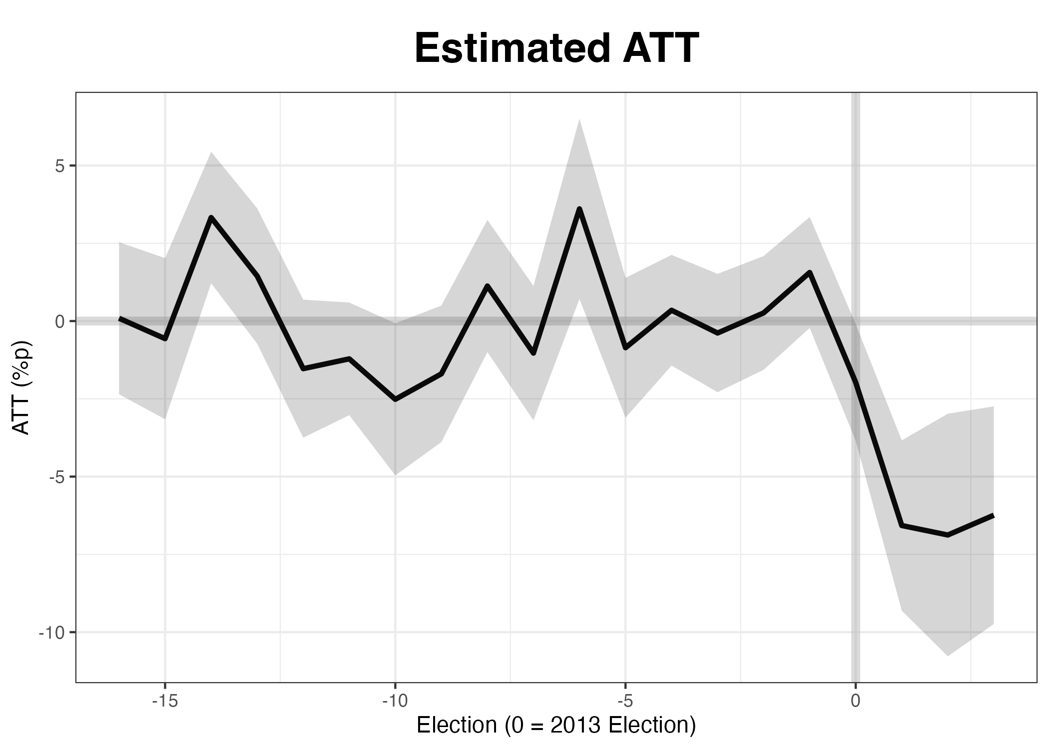
　以上の結果を可視化するためにはplot()関数を使う。タイトル、横軸、縦軸のラベルはmain、xlab、ylabで指定できる。

plot(scm_fit, 
     main = "Estimated ATT", 
     xlab = "Election (0 = 2013 Election)", 
     ylab = "ATT (%p)")

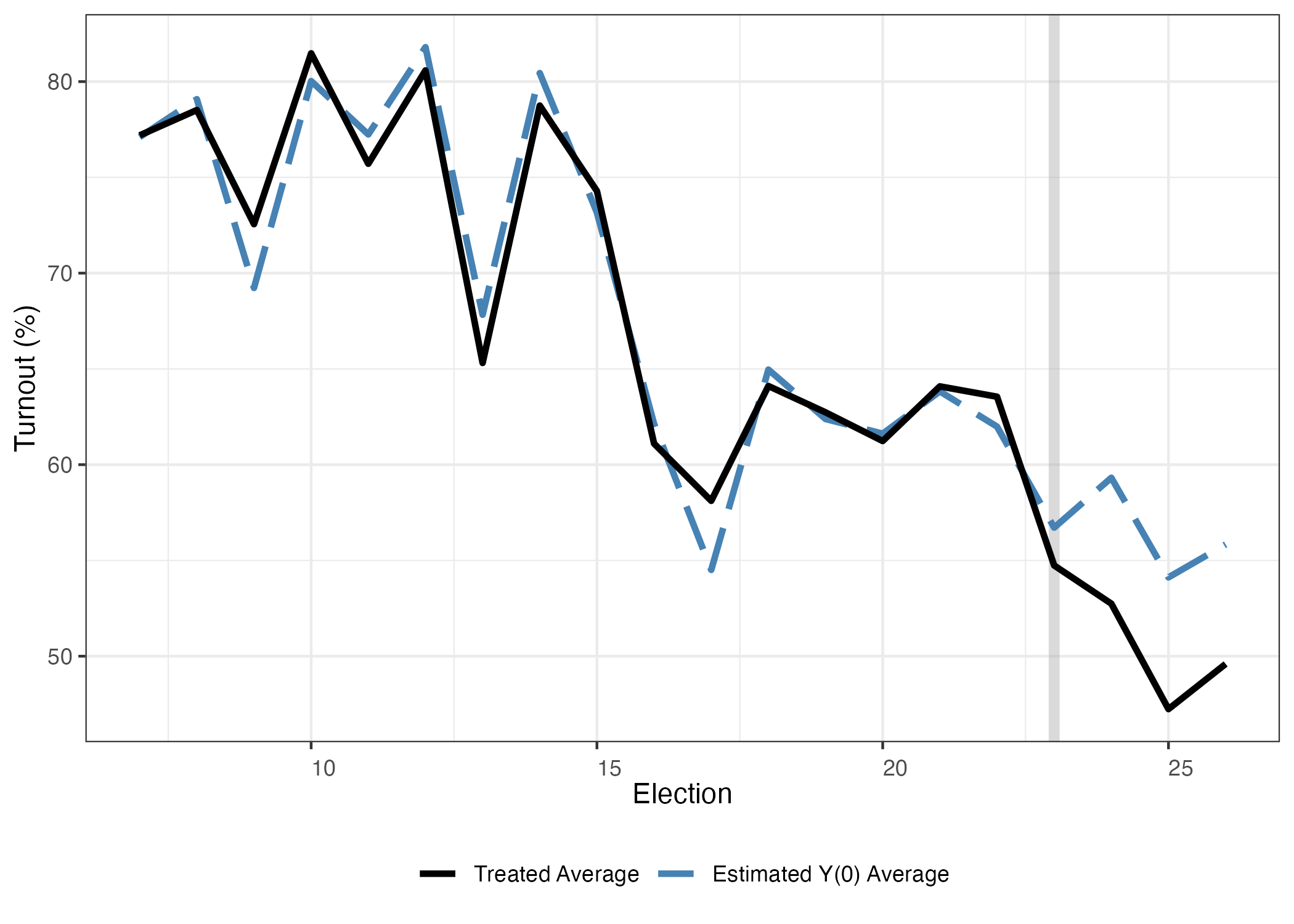
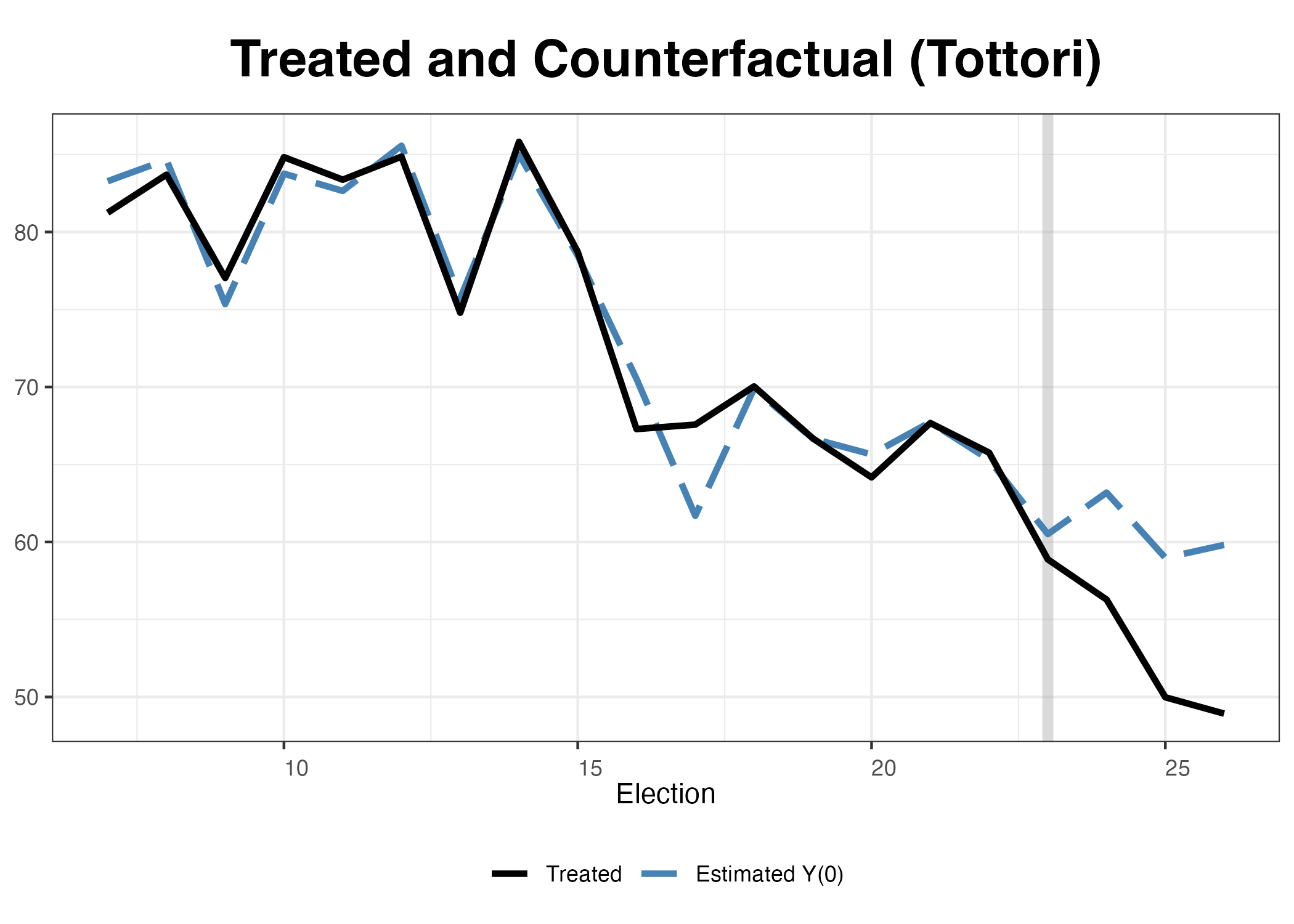
　処置を受ける前は架空の4県とその実際の4県の間に投票率の差はあまりなかったが、処置を受けてから差が広がることが分かる。差分でなく、合成された架空の4県と実際の4県のトレンドを見るためにはtype = "counterfactual"、もしくはtype = "ct"を指定します。

plot(scm_fit, 
     type = "counterfactual", 
     main = "",
     xlab = "Election", 
     ylab = "Turnout (%)")

　処置を受けたのは4県であるが、線が1本になっている。ここからも処置前は架空の4県と実際の4県はほぼ同じトレンドを示していますが、処置後は傾向が変わったことが確認できる。

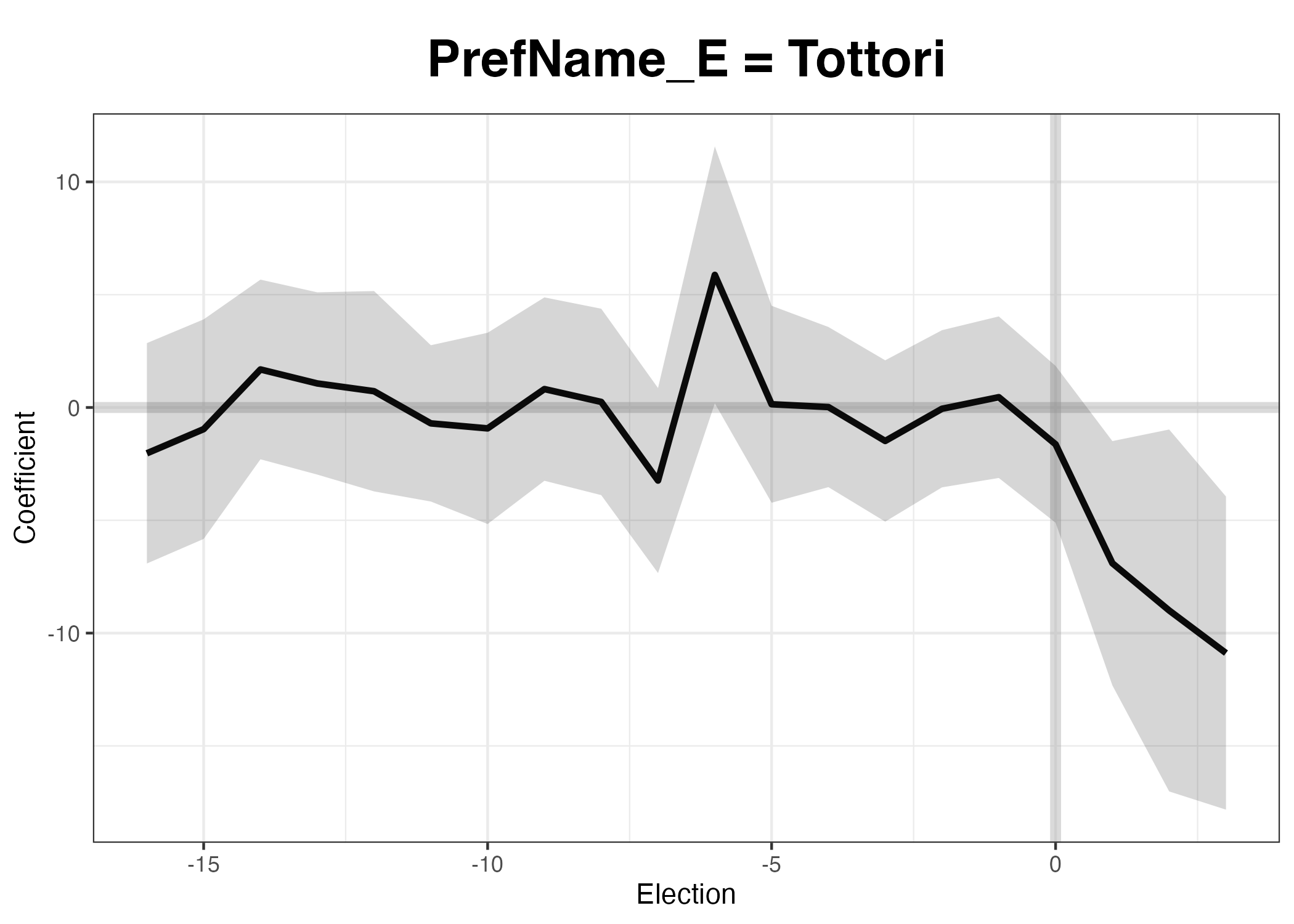
　もし、4つの都道府県を個別に示したい場合はどうすれば良いだろうか。この場合、plot()内にid引数を使えば良い。たとえば、鳥取県の処置効果（ATT）を確認するためにはid = "Tottori"と指定する。

plot(scm_fit, id = "Tottori")

plot(scm_fit, id = "Tottori", type = "ct")

　4つの都道府県のデータを個別のファセットで全て出すためにはゼロベースで作図した方が効率的かも知れない。また、この場合は図のカスタマイズの幅も広がる。{gsynth}から得られたオブジェクトには架空の鳥取、島根、徳島、高知のデータが個別に格納されているため、それを抽出すれば個別の図を作成することもできる。たとえば、処置群（4県）の観察済みのデータはオブジェクト名$Y.trで抽出できる。

scm_fit$Y.tr

      Kochi  Shimane Tokushima  Tottori
7  74.63966 83.49050  69.39499 81.24437
8  75.69312 84.78405  69.88441 83.69962
9  71.37616 78.14244  63.66989 77.03502
10 75.69410 86.92480  78.45754 84.82852
11 70.90031 85.15588  63.40844 83.37384
12 72.83410 87.58638  77.05070 84.86225
13 61.27247 75.36695  49.81165 74.79201
14 72.01185 86.89197  70.26960 85.81677
15 70.52034 82.31831  65.59127 78.71451
16 54.89730 73.79272  48.42299 67.28538
17 50.63857 67.09330  47.14380 67.57092
18 56.21296 73.26601  56.91326 70.03591
19 58.38653 68.61257  57.24322 66.68463
20 57.29701 68.87462  54.59808 64.16773
21 58.39998 71.80893  58.46591 67.67363
22 58.49266 71.70006  58.23675 65.76520
23 49.88987 60.89257  49.29437 58.87696
24 45.51522 62.19714  46.97798 56.28266
25 46.34053 54.04000  38.59305 49.97934
26 47.36311 56.37101  45.72428 48.92585

　このデータは行列構造となっているため、as_tibble()で表形式へ変更し、treat_dfという名で格納する。

treat_df <- as_tibble(scm_fit$Y.tr)

treat_df

# A tibble: 20 × 4
   Kochi Shimane Tokushima Tottori
   <dbl>   <dbl>     <dbl>   <dbl>
 1  74.6    83.5      69.4    81.2
 2  75.7    84.8      69.9    83.7
 3  71.4    78.1      63.7    77.0
 4  75.7    86.9      78.5    84.8
 5  70.9    85.2      63.4    83.4
 6  72.8    87.6      77.1    84.9
 7  61.3    75.4      49.8    74.8
 8  72.0    86.9      70.3    85.8
 9  70.5    82.3      65.6    78.7
10  54.9    73.8      48.4    67.3
11  50.6    67.1      47.1    67.6
12  56.2    73.3      56.9    70.0
13  58.4    68.6      57.2    66.7
14  57.3    68.9      54.6    64.2
15  58.4    71.8      58.5    67.7
16  58.5    71.7      58.2    65.8
17  49.9    60.9      49.3    58.9
18  45.5    62.2      47.0    56.3
19  46.3    54.0      38.6    50.0
20  47.4    56.4      45.7    48.9

　このtreat_dfだけは各投票率がいつの投票率かが分からない。Election列をKochi列前に追加し（mutate()内の最後に.before = Kochiを指定すると、mutate()で生成・修正された列がKochi列の前へ移動する）、7から26までを入れる。

treat_df <- treat_df |>
  mutate(Election = 7:26, .before = Kochi)

treat_df

# A tibble: 20 × 5
   Election Kochi Shimane Tokushima Tottori
      <int> <dbl>   <dbl>     <dbl>   <dbl>
 1        7  74.6    83.5      69.4    81.2
 2        8  75.7    84.8      69.9    83.7
 3        9  71.4    78.1      63.7    77.0
 4       10  75.7    86.9      78.5    84.8
 5       11  70.9    85.2      63.4    83.4
 6       12  72.8    87.6      77.1    84.9
 7       13  61.3    75.4      49.8    74.8
 8       14  72.0    86.9      70.3    85.8
 9       15  70.5    82.3      65.6    78.7
10       16  54.9    73.8      48.4    67.3
11       17  50.6    67.1      47.1    67.6
12       18  56.2    73.3      56.9    70.0
13       19  58.4    68.6      57.2    66.7
14       20  57.3    68.9      54.6    64.2
15       21  58.4    71.8      58.5    67.7
16       22  58.5    71.7      58.2    65.8
17       23  49.9    60.9      49.3    58.9
18       24  45.5    62.2      47.0    56.3
19       25  46.3    54.0      38.6    50.0
20       26  47.4    56.4      45.7    48.9

　続いて、{tidyr}のpivot_longer()関数を使ってtreat_dfをlong型データへ変換する。pivot_*()関数の使い方については『私たちのR』第15章「整然データ構造」を参照されたい。

treat_df <- treat_df |>
  pivot_longer(cols      = Kochi:Tottori,
               names_to  = "Pref",
               values_to = "Turnout")

treat_df

# A tibble: 80 × 3
   Election Pref      Turnout
      <int> <chr>       <dbl>
 1        7 Kochi        74.6
 2        7 Shimane      83.5
 3        7 Tokushima    69.4
 4        7 Tottori      81.2
 5        8 Kochi        75.7
 6        8 Shimane      84.8
 7        8 Tokushima    69.9
 8        8 Tottori      83.7
 9        9 Kochi        71.4
10        9 Shimane      78.1
# ℹ 70 more rows

　同じ作業を架空の処置群についても行う。架空の処置群はオブジェクト名$Y.ctで抽出できる。今回は全ての作業をパイプ演算子で繋ぎ、コードを効率化する。

counter_df <- scm_fit$Y.ct |>
  as_tibble() |>
  mutate(Election = 7:26, .before = Kochi) |>
  pivot_longer(cols      = Kochi:Tottori,
               names_to  = "Pref",
               values_to = "Turnout")

counter_df

# A tibble: 80 × 3
   Election Pref      Turnout
      <int> <chr>       <dbl>
 1        7 Kochi        73.5
 2        7 Shimane      84.0
 3        7 Tokushima    67.6
 4        7 Tottori      83.3
 5        8 Kochi        75.3
 6        8 Shimane      85.7
 7        8 Tokushima    70.7
 8        8 Tottori      84.7
 9        9 Kochi        65.6
10        9 Shimane      76.1
# ℹ 70 more rows

　最後にtreat_dfとcounter_dfを結合する。treat_dfの行なら"観測値"の値が、counter_dfの行なら"反実仮想"の値が付けられたTypeという列を追加し、このType列をfactor化する。要素の順番は"反実仮想"、"観測値"の順とする。

tr_ct_df <- bind_rows(list("観測値"   = treat_df, 
                           "反実仮想" = counter_df),
                      .id = "Type") |>
  mutate(Type = factor(Type, levels = c("反実仮想", "観測値")))

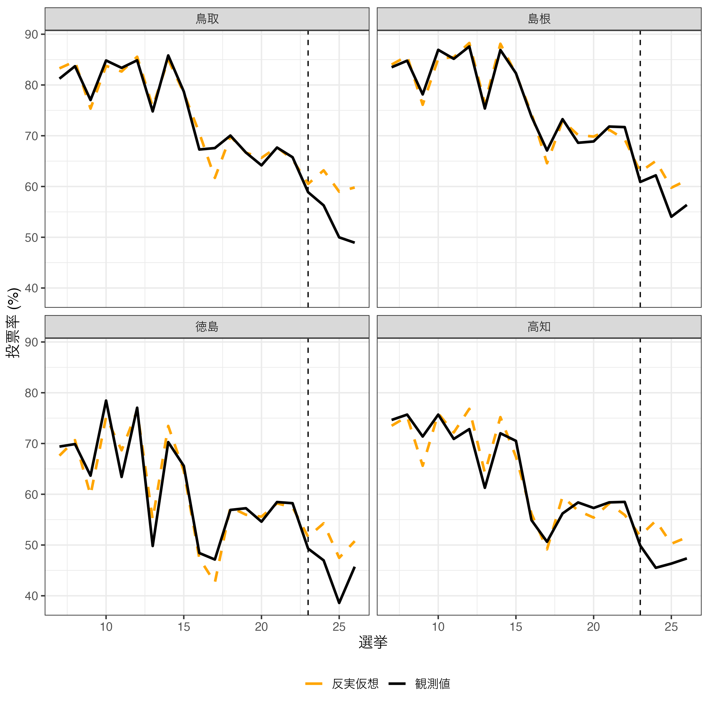
　データが揃ったので{ggplot2}を使って折れ線グラフを作ってみよう。

tr_ct_df |>
  # Pref列をリコーディング & factor化
  mutate(Pref = recode(Pref,
                       "Tottori"   = "鳥取",
                       "Shimane"   = "島根",
                       "Tokushima" = "徳島",
                       "Kochi"     = "高知"),
         Pref = factor(Pref, levels = c("鳥取", "島根", "徳島", "高知"))) |>
  ggplot() +
  # x = 23の箇所に垂直線の破線を引く
  geom_vline(xintercept = 23, linetype = 2) +
  geom_line(aes(x = Election, y = Turnout, linetype = Type, color = Type),
            size = 1) +
  # 線の色
  scale_color_manual(values = c("観測値"   = "black", 
                                "反実仮想" = "orange")) +
  # 線のタイプ（1 = 実線; 2 = 破線）
  scale_linetype_manual(values = c("観測値"   = 1, 
                                   "反実仮想" = 2)) +
  # colorの凡例は残し、linetypeの凡例は無くす
  guides(linetype = "none") +
  labs(x = "選挙", y = "投票率 (%)", color = "") +
  # 都道府県ごとにファセット分割
  facet_wrap(~Pref, ncol = 2) +
  theme_bw(base_size = 12) +
  theme(legend.position = "bottom")

　ただし、この図だけだと処置効果（ATT）が分かりにくい。処置効果は観測値（=処置群）と反実仮想（=架空の統制群）の差分である。tr_ct_dfからもATTの計算はできるが、ATTの不確実性（標準誤差や信頼区間など）までは分からない。処置効果（ATT）を抽出はオブジェクト名$est.indで出来るが、3次元配列（array構造）になっているため、オブジェクト名$est.ind[, , "処置群名"]で抽出する必要がある。処置群名は今回の場合だとPrefName_E上の名前である。たとえば、鳥取における処置効果は以下のように抽出する。これらもまた表形式でなく、行列構造であるので、as_tibble()を使って表形式にしよう。

as_tibble(scm_fit$est.ind[, , "Tottori"])

# A tibble: 20 × 5
        Eff  S.E. CI.lower CI.upper p.value
      <dbl> <dbl>    <dbl>    <dbl>   <dbl>
 1  -2.03    2.31   -6.56      2.50 0.379  
 2  -0.960   2.33   -5.53      3.61 0.681  
 3   1.69    2.06   -2.34      5.71 0.412  
 4   1.07    2.09   -3.03      5.16 0.610  
 5   0.721   2.01   -3.22      4.66 0.720  
 6  -0.704   1.73   -4.09      2.68 0.683  
 7  -0.926   2.08   -5.01      3.16 0.656  
 8   0.816   2.07   -3.25      4.88 0.694  
 9   0.247   2.02   -3.71      4.21 0.903  
10  -3.24    2.19   -7.52      1.05 0.138  
11   5.88    3.13   -0.252    12.0  0.0602 
12   0.143   2.14   -4.06      4.35 0.947  
13   0.0189  1.98   -3.86      3.90 0.992  
14  -1.48    1.76   -4.94      1.97 0.400  
15  -0.0566  1.72   -3.43      3.32 0.974  
16   0.456   1.71   -2.89      3.80 0.789  
17  -1.63    1.66   -4.88      1.61 0.324  
18  -6.90    2.63  -12.1      -1.75 0.00869
19  -9.00    3.98  -16.8      -1.20 0.0237 
20 -10.9     3.37  -17.5      -4.28 0.00123

　ここでEff列が架空の鳥取と実際の鳥取の差、つまり処置効果である。そして、CI.lowerとCI.upperがそれぞれ95%信頼区間の下限と上限だ。これら4つの県のデータを結合し、Election変数を追加、都道府県をfactor化したものをatt_dfという名で格納する。

att_df <- bind_rows(list("鳥取" = as_tibble(scm_fit$est.ind[, , "Tottori"]),
                         "島根" = as_tibble(scm_fit$est.ind[, , "Shimane"]),
                         "徳島" = as_tibble(scm_fit$est.ind[, , "Tokushima"]),
                         "高知" = as_tibble(scm_fit$est.ind[, , "Kochi"])),
                    .id = "Pref") |>
  mutate(Election = rep(7:26, 4), # 7~26を4回繰り返し
         .before = Pref) |>       # Election列をPref列の前に
  mutate(Pref = fct_inorder(Pref))

att_df

# A tibble: 80 × 7
   Election Pref     Eff  S.E. CI.lower CI.upper p.value
      <int> <fct>  <dbl> <dbl>    <dbl>    <dbl>   <dbl>
 1        7 鳥取  -2.03   2.31    -6.56     2.50   0.379
 2        8 鳥取  -0.960  2.33    -5.53     3.61   0.681
 3        9 鳥取   1.69   2.06    -2.34     5.71   0.412
 4       10 鳥取   1.07   2.09    -3.03     5.16   0.610
 5       11 鳥取   0.721  2.01    -3.22     4.66   0.720
 6       12 鳥取  -0.704  1.73    -4.09     2.68   0.683
 7       13 鳥取  -0.926  2.08    -5.01     3.16   0.656
 8       14 鳥取   0.816  2.07    -3.25     4.88   0.694
 9       15 鳥取   0.247  2.02    -3.71     4.21   0.903
10       16 鳥取  -3.24   2.19    -7.52     1.05   0.138
# ℹ 70 more rows

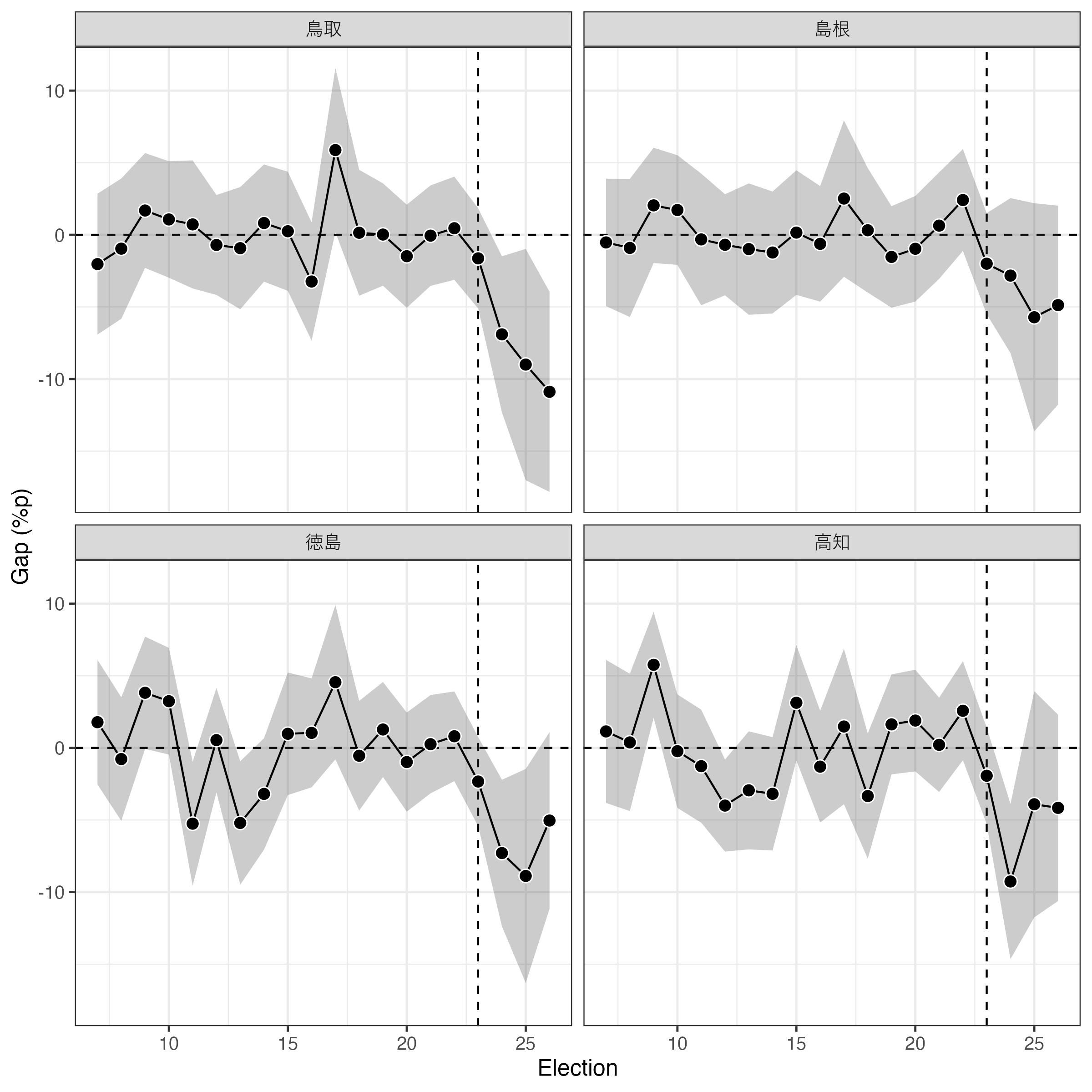
　それでは折れ線グラフを作ってみよう。ただし、今回は点推定値（折れ線グラフ）だけでなく、信頼区間も示す必要があるのでgeom_ribbon()レイヤーを追加する。

att_df |>
  ggplot() +
  geom_hline(yintercept = 0, linetype = 2) +
  geom_vline(xintercept = 23, linetype = 2) +
  # 信頼区間
  geom_ribbon(aes(x = Election, ymin = CI.lower, ymax = CI.upper),
              alpha = 0.25) +
  geom_line(aes(x = Election, y = Eff)) +
  # 以下のgeom_point()なあってもなくても良い
  geom_point(aes(x = Election, y = Eff), 
             size = 3, shape = 21, fill = "black", color = "white") +
  labs(x = "Election", y = "Gap (%p)") +
  facet_wrap(~Pref, ncol = 2) +
  theme_bw(base_size = 12) +
  theme(legend.position = "bottom")

　個別に見ると、合区直後、合区によって投票率を下がったのは鳥取、徳島、高知である。しかし、合区から3回目の選挙となる2022年（第26回）では鳥取のみとなる。

　SCMは統制群から合成された架空の鳥取、島根、徳島、高知を作成し、こちらを実際の統制群として用いる手法である。その際に43都道府県を重み付け合成されるが、それぞれの重みはいくつだろうか。gsynth()から得られたオブジェクトからwgt.impliedを抽出すればその重みが分かる。通常のSCMの場合、重みは正の値であるが、一般化SCMの場合は負も正もあり得る。

scm_fit$wgt.implied

	Kochi	Shimane	Tokushima	Tottori
Aichi	0.022	−2.169	−2.755	0.448
Akita	−0.151	−0.161	−0.798	0.170
Aomori	−0.069	−1.188	−1.613	0.225
Chiba	0.309	−2.096	−1.885	0.327
Ehime	0.238	0.471	0.851	−0.009
Fukui	−0.630	4.081	4.711	−1.122
Fukuoka	−0.541	0.634	0.342	−0.368
Fukushima	0.947	−0.235	0.669	0.402
Gifu	0.354	0.149	0.566	0.097
Gunma	0.318	2.085	2.968	−0.291
Hiroshima	−0.254	1.622	2.146	−0.570
Hokkaido	−0.553	−3.254	−5.161	0.643
Hyogo	0.117	−3.045	−3.918	0.723
Ibaraki	0.378	−0.483	0.902	−0.263
Ishikawa	−0.480	1.476	1.294	−0.432
Iwate	0.006	−2.615	−4.020	0.833
Kagawa	−0.391	3.227	3.960	−0.902
Kagoshima	0.098	0.202	−0.102	0.200
Kanagawa	0.506	−3.426	−3.741	0.828
Kumamoto	−0.791	1.767	1.083	−0.490
Kyoto	0.397	−4.141	−5.373	1.200
Mie	0.016	−1.162	−1.447	0.231
Miyagi	0.712	−0.122	1.072	0.070
Miyazaki	−1.071	5.630	6.465	−1.699
Nagano	0.498	−1.419	−1.244	0.446
Nagasaki	−0.921	1.910	1.572	−0.763
Nara	0.378	−2.473	−2.658	0.589
Nigata	0.856	−2.080	−1.318	0.535
Oita	−0.593	2.253	1.749	−0.444
Okayama	−0.264	0.966	1.560	−0.557
Okinawa	0.958	0.416	0.697	0.637
Osaka	0.387	−3.404	−4.601	1.118
Saga	−0.913	4.668	5.637	−1.552
Saitama	0.217	−0.975	−0.328	−0.031
Shiga	−0.012	−0.073	−0.613	0.235
Shizuoka	0.599	0.961	2.654	−0.330
Tochigi	0.409	0.338	1.366	−0.143
Tokyo	0.619	−4.424	−5.420	1.301
Toyama	−0.819	4.384	5.389	−1.467
Wakayama	−0.050	−1.103	−1.730	0.323
Yamagata	0.652	−1.077	−0.815	0.508
Yamaguchi	−1.048	1.821	0.402	−0.382
Yamanashi	−0.444	2.064	1.486	−0.274

脚注

fixed_effects引数でなく、回帰式に説明変数として指定しても結果は同じである。しかし、回帰式に書く場合、固定効果の推定値も全て出力され、推定結果が非常に長くなる。しかし、固定効果の推定値は論文内で報告することもない。fixed_effectsで指定すると、それらの結果は省略される。↩︎
{gsynth}は通常のSCMでなく、一般化SCM（Generalized Synthetic Control Method）を実装したパッケージである。通常のSCMは処置群は1つのみに使えるが、一般化SCMは処置群が複数あっても使える。一般化SCMについてはYiqing Xu. 2017. “Generalized Synthetic Control Method: Causal Inference with Interactive Fixed Effects Models,” Political Analysis, 25 (1): 57-76.を参照されたい。↩︎
第7〜23回参院選のデータは参議院議員通常選挙データベースからダウンロードしたものを架空したものであり、第24〜26回データは宋が手入力したものである。↩︎