セットアップ
本日の実習に必要なパッケージとデータを読み込む。
:: p_load (tidyverse, # Rの必須パッケージ # 記述統計 # 推定結果の要約 # ロバストな回帰分析 <- read_csv ("data/did_data3.csv" )
# A tibble: 18,749 × 14
   county state  year shooting fatal_shooting non_fatal_shooting turnout demvote
    <dbl> <chr> <dbl>    <dbl>          <dbl>              <dbl>   <dbl>   <dbl>
 1   1001 01     1996        0              0                  0    56.1    32.5
 2   1001 01     2000        0              0                  0    56.8    28.7
 3   1001 01     2004        0              0                  0    60.2    23.7
 4   1001 01     2008        0              0                  0    64.1    25.8
 5   1001 01     2012        0              0                  0    61.0    26.5
 6   1001 01     2016        0              0                  0    60.7    24.0
 7   1003 01     1996        0              0                  0    51.8    27.1
 8   1003 01     2000        0              0                  0    54.6    24.8
 9   1003 01     2004        0              0                  0    59.8    22.5
10   1003 01     2008        0              0                  0    62.4    23.8
# ℹ 18,739 more rows
# ℹ 6 more variables: population <dbl>, non_white <dbl>,
#   change_unem_rate <dbl>, county_f <dbl>, state_f <chr>, year_f <dbl>
データの詳細はスライドを参照すること。DID推定には時間(年)とカウンティー(郡)の固定効果を投入し、州レベルでクラスタリングした標準誤差を使う予定である。これらの変数を予めfactor化しておこう。factor化した変数は変数名の後ろに_fを付けて、新しい列として追加しておく。
<- did_df |> mutate (county_f = factor (county),state_f = factor (state),year_f = factor (year))
# A tibble: 18,749 × 14
   county state  year shooting fatal_shooting non_fatal_shooting turnout demvote
    <dbl> <chr> <dbl>    <dbl>          <dbl>              <dbl>   <dbl>   <dbl>
 1   1001 01     1996        0              0                  0    56.1    32.5
 2   1001 01     2000        0              0                  0    56.8    28.7
 3   1001 01     2004        0              0                  0    60.2    23.7
 4   1001 01     2008        0              0                  0    64.1    25.8
 5   1001 01     2012        0              0                  0    61.0    26.5
 6   1001 01     2016        0              0                  0    60.7    24.0
 7   1003 01     1996        0              0                  0    51.8    27.1
 8   1003 01     2000        0              0                  0    54.6    24.8
 9   1003 01     2004        0              0                  0    59.8    22.5
10   1003 01     2008        0              0                  0    62.4    23.8
# ℹ 18,739 more rows
# ℹ 6 more variables: population <dbl>, non_white <dbl>,
#   change_unem_rate <dbl>, county_f <fct>, state_f <fct>, year_f <fct>
連続変数(shootingからchange_unem_rateまで)の記述統計量を出力する。ここで一つ注意が必要だ。それはselect()関数の使い方である。具体的に言えば、使い方そのものは変わらない。
|> select (shooting: change_unem_rate) |> descr (stats = c ("mean" , "sd" , "min" , "max" , "n.valid" ),transpose = TRUE , order = "p" )
Descriptive Statistics
did_df
N: 18749

                               Mean     Std.Dev      Min           Max    N.Valid
------------------------ ---------- ----------- -------- ------------- ----------
                shooting       0.00        0.07     0.00          1.00   18749.00
          fatal_shooting       0.00        0.05     0.00          1.00   18749.00
      non_fatal_shooting       0.00        0.04     0.00          1.00   18749.00
                 turnout      57.94       10.32     1.08        300.00   18627.00
                 demvote      39.01       13.79     3.14         92.85   18627.00
              population   95121.69   306688.63    55.00   10137915.00   18749.00
               non_white       0.13        0.16     0.00          0.96   18749.00
        change_unem_rate      -0.39        2.34   -19.60         15.30   18749.00
Diff-in-Diff
それでは差分の差分法の実装について紹介する。推定式は以下の通りである。
\[
\mbox{Outcome}_{i, t} = \beta_0 + \beta_1 \mbox{Shooting}_{i, t} + \sum_k \delta_{k, i, t} \mbox{Controls}_{k, i, t} + \lambda_{t} + \omega_{i} + \varepsilon_{i, t}
\]
\(\mbox{Otucome}\) : 応答変数
turnout: 投票率(大統領選挙)demvote: 民主党候補者の得票率 \(\mbox{Shooting}\) : 処置変数
shooting: 銃撃事件の発生有無fatal_shooting: 死者を伴う銃撃事件の発生有無non_fatal_shooting: 死者を伴わない銃撃事件の発生有無 \(\mbox{Controls}\) : 統制変数
population: カウンティーの人口non_white: 非白人の割合change_unem_rate: 失業率の変化統制変数あり/なしのモデルを個別に推定
\(\lambda\) : 年固定効果\(\omega\) : カウンティー固定効果
応答変数が2種類、処置変数が3種類、共変量の有無でモデルを分けるので、推定するモデルは計12個である。
モデル1
did_fit1turnoutshootingなし
モデル2
did_fit2turnoutshootingあり
モデル3
did_fit3turnoutfatal_shootingなし
モデル4
did_fit4turnoutfatal_shootingあり
モデル5
did_fit5turnoutnon_fatal_shootingなし
モデル6
did_fit6turnoutnon_fatal_shootingあり
モデル7
did_fit7demvoteshootingなし
モデル8
did_fit8demvoteshootingあり
モデル9
did_fit9demvotefatal_shootingなし
モデル10
did_fit10demvotefatal_shootingあり
モデル11
did_fit11demvotenon_fatal_shootingなし
モデル12
did_fit12demvotenon_fatal_shootingあり
まずはモデル1を推定し、did_fit1という名のオブジェクトとして格納する。基本的には線形回帰分析であるため、lm()でも推定はできる。しかし、差分の差分法の場合、通常、クラスター化した頑健な標準誤差(cluster robust standard error)を使う。lm()単体ではこれが計算できないため、今回は{estimatr}パッケージが提供するlm_robust()関数を使用する。使い方はlm()同様、まず回帰式と使用するデータ名を指定する。続いて、固定効果をfixed_effects引数で指定する。書き方は~固定効果変数1 + 固定効果変数2 + ...である。回帰式と違って、~の左側には変数がないことに注意すること。続いて、clusters引数でクラスタリングする変数を指定する。今回は州レベルでクラスタリングするので、state_fで良い。最後に標準誤差のタイプを指定するが、デフォルトは"CR2"となっている。今回のデータはそれなりの大きさのデータであり、"CR2"だと推定時間が非常に長くなる。ここでは推定時間が比較的早い"stata"とする。
<- lm_robust (turnout ~ shooting, data = did_df, fixed_effects = ~ year_f + county_f,clusters = state_f,se_type = "stata" )summary (did_fit1)
Call:
lm_robust(formula = turnout ~ shooting, data = did_df, clusters = state_f,
    fixed_effects = ~year_f + county_f, se_type = "stata")

Standard error type:  stata

Coefficients:
         Estimate Std. Error t value Pr(>|t|) CI Lower CI Upper DF
shooting  -0.5211     0.6457  -0.807   0.4235   -1.819   0.7764 49

Multiple R-squared:  0.8575 ,   Adjusted R-squared:  0.8288
Multiple R-squared (proj. model):  6.907e-05 ,  Adjusted R-squared (proj. model):  -0.2008
F-statistic (proj. model): 0.6513 on 1 and 49 DF,  p-value: 0.4235
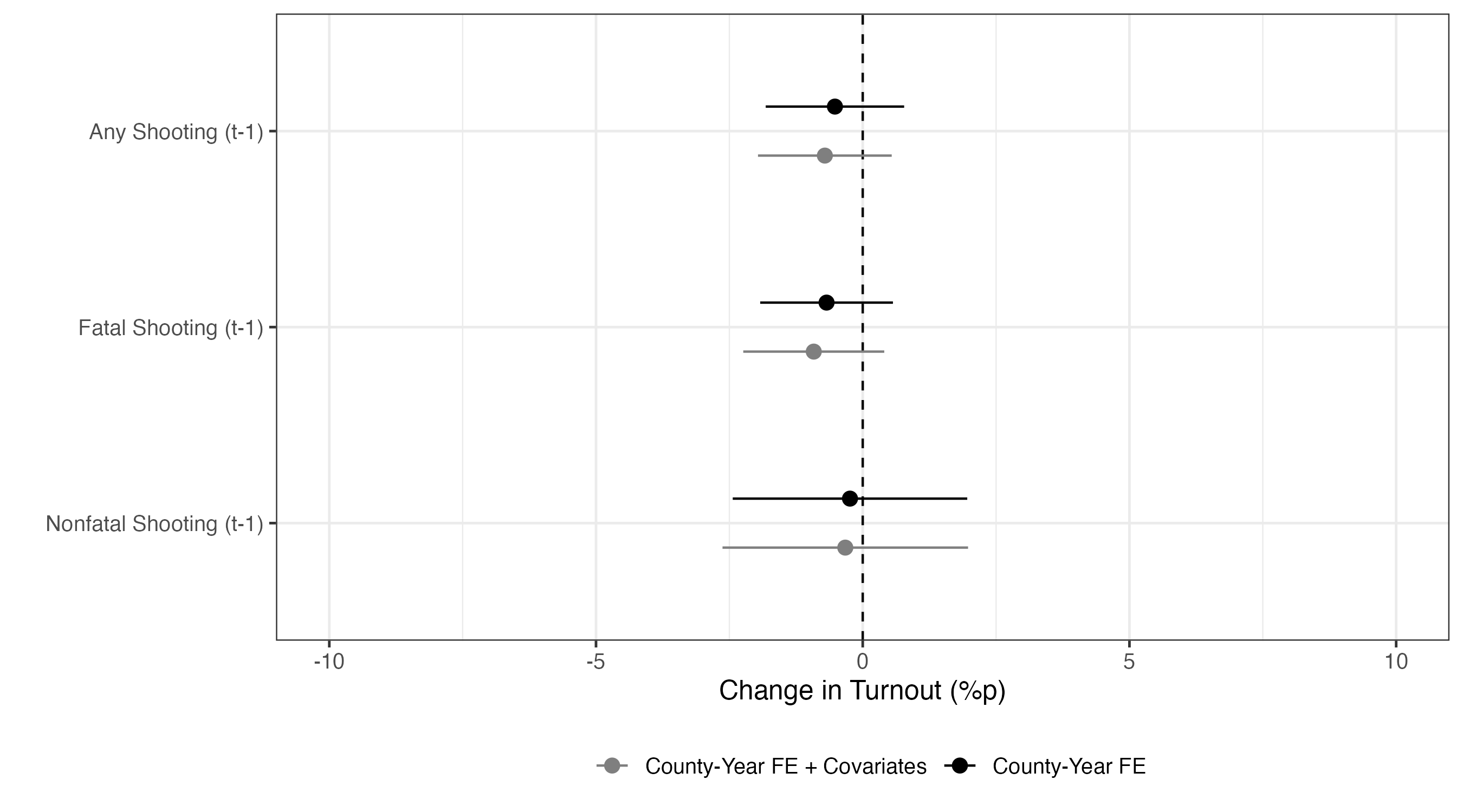
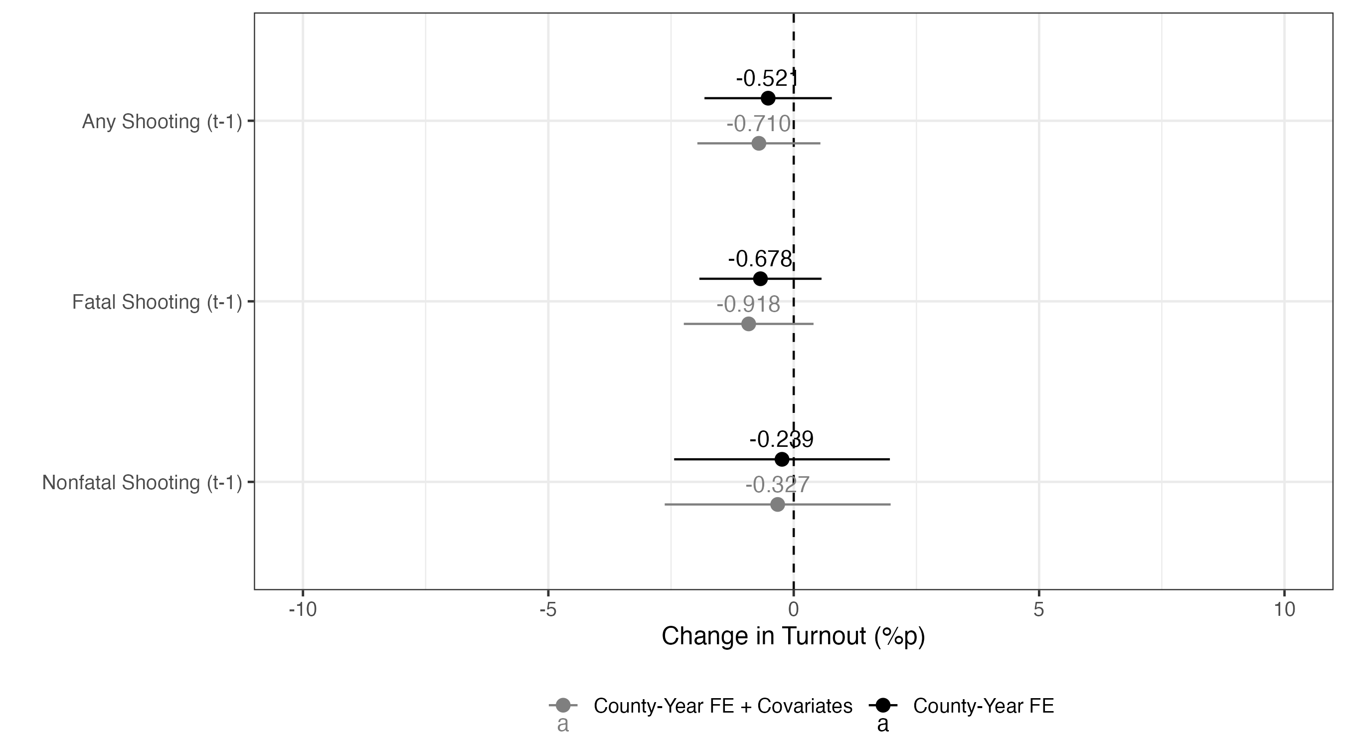
処置効果の推定値は-0.521である。これは学校内銃撃事件が発生したカウンティーの場合、大統領選挙において投票率が約-0.521%p低下することを意味する。しかし、標準誤差がかなり大きく、統計的有意な結果ではない。つまり、「学校内銃撃事件が投票率を上げる(or 下げる)とは言えない」と解釈できる。決して「学校内銃撃事件が投票率を上げない(or 下げない)」と解釈しないこと。
共変量を投入してみたらどうだろうか。たとえば、人口は自治体の都市化程度を表すこともあるので、都市化程度と投票率には関係があると考えられる。また、人口が多いと自然に事件が発生する確率もあがるので、交絡要因として考えられる。人種や失業率も同様であろう。ここではカウンティーの人口(population)、非白人の割合(non_white)、失業率の変化(change_unem_rate)を統制変数として投入し、did_fit2という名で格納する。
<- lm_robust (turnout ~ shooting + + non_white + change_unem_rate, data = did_df, fixed_effects = ~ year_f + county_f,clusters = state_f,se_type = "stata" )summary (did_fit2)
Call:
lm_robust(formula = turnout ~ shooting + population + non_white +
    change_unem_rate, data = did_df, clusters = state_f, fixed_effects = ~year_f +
    county_f, se_type = "stata")

Standard error type:  stata

Coefficients:
                   Estimate Std. Error t value Pr(>|t|)   CI Lower   CI Upper
shooting         -7.098e-01  6.237e-01  -1.138  0.26066 -1.963e+00  5.436e-01
population        8.029e-06  5.688e-06   1.411  0.16443 -3.402e-06  1.946e-05
non_white        -3.483e+01  1.558e+01  -2.236  0.02990 -6.613e+01 -3.534e+00
change_unem_rate  1.592e-01  6.584e-02   2.418  0.01938  2.688e-02  2.915e-01
                 DF
shooting         49
population       49
non_white        49
change_unem_rate 49

Multiple R-squared:  0.8598 ,   Adjusted R-squared:  0.8316
Multiple R-squared (proj. model):  0.01669 ,    Adjusted R-squared (proj. model):  -0.1811
F-statistic (proj. model): 5.047 on 4 and 49 DF,  p-value: 0.001739
処置効果の推定値は-0.710である。これは他の条件が同じ場合、学校内銃撃事件が発生したカウンティーは大統領選挙において投票率が約-0.710%p低下することを意味する。ちなみに、e-01は\(\times 10^{-1}\) を、e-06は\(\times 10^{-6}\) を、e+01は\(\times 10^{1}\) 意味する。今回も統計的に非有意な結果が得られている。
これまでの処置変数は死者の有無と関係なく、学校内銃撃事件が発生したか否かだった。もしかしたら、死者を伴う銃撃事件が発生した場合、その効果が大きいかも知れない。したがって、これからは処置変数を死者を伴う学校内銃撃事件の発生有無(fatal_shooting)、死者を伴わない学校内銃撃事件の発生有無(non_fatal_shooting)に変えてもう一度推定してみよう。
<- lm_robust (turnout ~ fatal_shooting, data = did_df, fixed_effects = ~ year_f + county_f,clusters = state_f,se_type = "stata" )<- lm_robust (turnout ~ fatal_shooting + + non_white + change_unem_rate, data = did_df, fixed_effects = ~ year_f + county_f,clusters = state_f,se_type = "stata" )<- lm_robust (turnout ~ non_fatal_shooting, data = did_df, fixed_effects = ~ year_f + county_f,clusters = state_f,se_type = "stata" )<- lm_robust (turnout ~ non_fatal_shooting + + non_white + change_unem_rate, data = did_df, fixed_effects = ~ year_f + county_f,clusters = state_f,se_type = "stata" )
これまで推定してきた6つのモデルを比較してみよう。
modelsummary (list (did_fit1, did_fit2, did_fit3,
(1)
(2)
(3)
(4)
(5)
(6)
shooting
-0.521
-0.710
(0.646)
(0.624)
population
0.000
0.000
0.000
(0.000)
(0.000)
(0.000)
non_white
-34.834
-34.844
-34.814
(15.575)
(15.618)
(15.614)
change_unem_rate
0.159
0.159
0.160
(0.066)
(0.066)
(0.066)
fatal_shooting
-0.678
-0.918
(0.619)
(0.658)
non_fatal_shooting
-0.239
-0.327
(1.094)
(1.145)
Num.Obs.
18627
18627
18627
18627
18627
18627
R2
0.857
0.860
0.857
0.860
0.857
0.860
R2 Adj.
0.829
0.832
0.829
0.832
0.829
0.832
AIC
103543.4
103237.2
103543.3
103237.1
103544.6
103239.4
BIC
103559.0
103276.4
103559.0
103276.3
103560.2
103278.6
RMSE
3.90
3.87
3.90
3.87
3.90
3.87
Std.Errors
by: state_f
by: state_f
by: state_f
by: state_f
by: state_f
by: state_f
いずれのモデルも統計的に有意な処置効果は確認されていない。これらの結果を表として報告するには紙がもったいない気もする。これらの結果はOnline Appendixに回し、本文中には処置効果の点推定値と95%信頼区間を示せば良いだろう。
{broom}のtidy()関数で推定結果のみを抽出し、それぞれオブジェクトとして格納しておこう。
<- tidy (did_fit1, conf.int = TRUE )<- tidy (did_fit2, conf.int = TRUE )<- tidy (did_fit3, conf.int = TRUE )<- tidy (did_fit4, conf.int = TRUE )<- tidy (did_fit5, conf.int = TRUE )<- tidy (did_fit6, conf.int = TRUE )
全て確認する必要はないので、tidy_fit1のみを確認してみる。
      term   estimate std.error  statistic   p.value conf.low conf.high df
1 shooting -0.5210841 0.6456718 -0.8070417 0.4235426 -1.81861  0.776442 49
  outcome
1 turnout
以上の6つの表形式オブジェクトを一つの表としてまとめる。それぞれのオブジェクトには共変量の有無_処置変数の種類の名前を付けよう。共変量なしのモデルはM1、ありのモデルはM2とする。処置変数はshootingの場合はTr1、fatal_shootingはTr2、non_fatal_shootingはTr3とする。
<- bind_rows (list ("M1_Tr1" = tidy_fit1,"M2_Tr1" = tidy_fit2,"M1_Tr2" = tidy_fit3,"M2_Tr2" = tidy_fit4,"M1_Tr3" = tidy_fit5,"M2_Tr3" = tidy_fit6),.id = "Model" )
    Model               term      estimate    std.error  statistic    p.value
1  M1_Tr1           shooting -5.210841e-01 6.456718e-01 -0.8070417 0.42354260
2  M2_Tr1           shooting -7.097922e-01 6.237320e-01 -1.1379763 0.26066411
3  M2_Tr1         population  8.028568e-06 5.688141e-06  1.4114574 0.16442833
4  M2_Tr1          non_white -3.483443e+01 1.557543e+01 -2.2364985 0.02990378
5  M2_Tr1   change_unem_rate  1.592020e-01 6.584450e-02  2.4178480 0.01937671
6  M1_Tr2     fatal_shooting -6.779229e-01 6.191749e-01 -1.0948810 0.27892152
7  M2_Tr2     fatal_shooting -9.179995e-01 6.576559e-01 -1.3958659 0.16904785
8  M2_Tr2         population  8.026778e-06 5.747531e-06  1.3965611 0.16883977
9  M2_Tr2          non_white -3.484436e+01 1.561829e+01 -2.2309975 0.03029042
10 M2_Tr2   change_unem_rate  1.591126e-01 6.591001e-02  2.4140886 0.01955574
11 M1_Tr3 non_fatal_shooting -2.387205e-01 1.093832e+00 -0.2182423 0.82814672
12 M2_Tr3 non_fatal_shooting -3.269742e-01 1.145303e+00 -0.2854915 0.77647098
13 M2_Tr3         population  7.821482e-06 5.712400e-06  1.3692110 0.17717684
14 M2_Tr3          non_white -3.481384e+01 1.561438e+01 -2.2296020 0.03038921
15 M2_Tr3   change_unem_rate  1.595359e-01 6.590170e-02  2.4208169 0.01923637
        conf.low     conf.high df outcome
1  -1.818610e+00  7.764420e-01 49 turnout
2  -1.963229e+00  5.436442e-01 49 turnout
3  -3.402178e-06  1.945932e-05 49 turnout
4  -6.613442e+01 -3.534428e+00 49 turnout
5   2.688251e-02  2.915215e-01 49 turnout
6  -1.922202e+00  5.663557e-01 49 turnout
7  -2.239609e+00  4.036096e-01 49 turnout
8  -3.523318e-06  1.957687e-05 49 turnout
9  -6.623047e+01 -3.458237e+00 49 turnout
10  2.666148e-02  2.915637e-01 49 turnout
11 -2.436859e+00  1.959418e+00 49 turnout
12 -2.628546e+00  1.974598e+00 49 turnout
13 -3.658017e-06  1.930098e-05 49 turnout
14 -6.619211e+01 -3.435580e+00 49 turnout
15  2.710152e-02  2.919704e-01 49 turnout
続いて、処置効果のみを抽出する。処置効果はterm列の値が"shooting"、"fatal_shooting"、"non_fatal_shooting"のいずれかと一致する行であるため、filter()関数を使用する。
<- did_est1 |> filter (term %in% c ("shooting" , "fatal_shooting" , "non_fatal_shooting" ))
   Model               term   estimate std.error  statistic   p.value  conf.low
1 M1_Tr1           shooting -0.5210841 0.6456718 -0.8070417 0.4235426 -1.818610
2 M2_Tr1           shooting -0.7097922 0.6237320 -1.1379763 0.2606641 -1.963229
3 M1_Tr2     fatal_shooting -0.6779229 0.6191749 -1.0948810 0.2789215 -1.922202
4 M2_Tr2     fatal_shooting -0.9179995 0.6576559 -1.3958659 0.1690478 -2.239609
5 M1_Tr3 non_fatal_shooting -0.2387205 1.0938325 -0.2182423 0.8281467 -2.436859
6 M2_Tr3 non_fatal_shooting -0.3269742 1.1453027 -0.2854915 0.7764710 -2.628546
  conf.high df outcome
1 0.7764420 49 turnout
2 0.5436442 49 turnout
3 0.5663557 49 turnout
4 0.4036096 49 turnout
5 1.9594182 49 turnout
6 1.9745977 49 turnout
ちなみにgrepl()関数を使うと、"shooting"が含まれる行を抽出することもできる。以下のコードは上記のコードと同じ機能をする。
<- did_est1 |> filter (grepl ("shooting" , term))
つづいて、Model列をModelとTreat列へ分割する。
<- did_est1 |> separate (col = Model,into = c ("Model" , "Treat" ),sep = "_" )
  Model Treat               term   estimate std.error  statistic   p.value
1    M1   Tr1           shooting -0.5210841 0.6456718 -0.8070417 0.4235426
2    M2   Tr1           shooting -0.7097922 0.6237320 -1.1379763 0.2606641
3    M1   Tr2     fatal_shooting -0.6779229 0.6191749 -1.0948810 0.2789215
4    M2   Tr2     fatal_shooting -0.9179995 0.6576559 -1.3958659 0.1690478
5    M1   Tr3 non_fatal_shooting -0.2387205 1.0938325 -0.2182423 0.8281467
6    M2   Tr3 non_fatal_shooting -0.3269742 1.1453027 -0.2854915 0.7764710
   conf.low conf.high df outcome
1 -1.818610 0.7764420 49 turnout
2 -1.963229 0.5436442 49 turnout
3 -1.922202 0.5663557 49 turnout
4 -2.239609 0.4036096 49 turnout
5 -2.436859 1.9594182 49 turnout
6 -2.628546 1.9745977 49 turnout
可視化に入る前にModel列とTreat列の値を修正する。Model列の値が"M1"なら"County-Year FE"に、それ以外なら"County-Year FE + Covariates"とリコーディングする。戻り値が2種類だからif_else()を使う。Treat列の場合、戻り値が3つなので、recode()かcase_when()を使う。ここではrecode()を使ってリコーディングする。最後にModelとTreatを表示順番でfactor化し(fct_inorder())、更に順番を逆転する(fct_rev())。
<- did_est1 |> mutate (Model = if_else (Model == "M1" ,"County-Year FE" , "County-Year FE + Covariates" ),Treat = recode (Treat,"Tr1" = "Any Shooting (t-1)" ,"Tr2" = "Fatal Shooting (t-1)" ,"Tr3" = "Nonfatal Shooting (t-1)" ),Model = fct_rev (fct_inorder (Model)),Treat = fct_rev (fct_inorder (Treat)))
                        Model                   Treat               term
1              County-Year FE      Any Shooting (t-1)           shooting
2 County-Year FE + Covariates      Any Shooting (t-1)           shooting
3              County-Year FE    Fatal Shooting (t-1)     fatal_shooting
4 County-Year FE + Covariates    Fatal Shooting (t-1)     fatal_shooting
5              County-Year FE Nonfatal Shooting (t-1) non_fatal_shooting
6 County-Year FE + Covariates Nonfatal Shooting (t-1) non_fatal_shooting
    estimate std.error  statistic   p.value  conf.low conf.high df outcome
1 -0.5210841 0.6456718 -0.8070417 0.4235426 -1.818610 0.7764420 49 turnout
2 -0.7097922 0.6237320 -1.1379763 0.2606641 -1.963229 0.5436442 49 turnout
3 -0.6779229 0.6191749 -1.0948810 0.2789215 -1.922202 0.5663557 49 turnout
4 -0.9179995 0.6576559 -1.3958659 0.1690478 -2.239609 0.4036096 49 turnout
5 -0.2387205 1.0938325 -0.2182423 0.8281467 -2.436859 1.9594182 49 turnout
6 -0.3269742 1.1453027 -0.2854915 0.7764710 -2.628546 1.9745977 49 turnout
それでは{ggplot2}を使ってpoint-rangeプロットを作成してみよう。
|> ggplot () + # x = 0の箇所に垂直線を引く。垂直線は破線(linetype = 2)とする。 geom_vline (xintercept = 0 , linetype = 2 ) + geom_pointrange (aes (x = estimate, xmin = conf.low, xmax = conf.high,y = Treat, color = Model),position = position_dodge2 (1 / 2 )) + labs (x = "Change in Turnout (%p)" , y = "" , color = "" ) + # 色を指定する。 # Modelの値が County-Year FE なら黒、 # County-Year FE + Covariates ならグレー、 scale_color_manual (values = c ("County-Year FE" = "black" , "County-Year FE + Covariates" = "gray50" )) + # 横軸の下限と上限を-10〜10とする。 coord_cartesian (xlim = c (- 10 , 10 )) + theme_bw (base_size = 12 ) + theme (legend.position = "bottom" )
元の論文を見ると、点の上に点推定値が書かれているが、私たちもこれを真似してみよう。文字列をプロットするレイヤーはgeom_text()とgeom_label()、annotate()があるが、ここではgeom_text()を使用する。文字列が表示される横軸上の位置(x)と縦軸上の位置(y)、そして出力する文字列(label)をマッピングする。点推定値は3桁まで出力したいので、sprintf()を使って、3桁に丸める。ただし、これだけだと点と文字が重なってしまう。vjustを-0.75にすることで、出力する文字列を点の位置を上の方向へ若干ずらすことができる。
|> ggplot () + geom_vline (xintercept = 0 , linetype = 2 ) + geom_pointrange (aes (x = estimate, xmin = conf.low, xmax = conf.high,y = Treat, color = Model),position = position_dodge2 (1 / 2 )) + geom_text (aes (x = estimate, y = Treat, color = Model, label = sprintf ("%.3f" , estimate)),position = position_dodge2 (1 / 2 ),vjust = - 0.75 ) + labs (x = "Change in Turnout (%p)" , y = "" , color = "" ) + scale_color_manual (values = c ("County-Year FE" = "black" , "County-Year FE + Covariates" = "gray50" )) + coord_cartesian (xlim = c (- 10 , 10 )) + theme_bw (base_size = 12 ) + theme (legend.position = "bottom" )
ちなみにこのコードを見ると、geom_pointrange()とgeom_text()はx、y、colorを共有しているので、ggplot()内でマッピングすることもできる。
|> ggplot (aes (x = estimate, y = Treat, color = Model)) + geom_vline (xintercept = 0 , linetype = 2 ) + geom_pointrange (aes (xmin = conf.low, xmax = conf.high),position = position_dodge2 (1 / 2 )) + geom_text (aes (label = sprintf ("%.3f" , estimate)),position = position_dodge2 (1 / 2 ),vjust = - 0.75 ) + labs (x = "Change in Turnout (%p)" , y = "" , color = "" ) + scale_color_manual (values = c ("County-Year FE" = "black" , "County-Year FE + Covariates" = "gray50" )) + coord_cartesian (xlim = c (- 10 , 10 )) + theme_bw (base_size = 12 ) + theme (legend.position = "bottom" )
続いて、民主党候補者の得票率(demvote)を応答変数として6つのモデルを推定し、同じ作業を繰り返す。
<- lm_robust (demvote ~ shooting, data = did_df, fixed_effects = ~ year_f + county_f,clusters = state_f,se_type = "stata" )<- lm_robust (demvote ~ shooting + + non_white + change_unem_rate, data = did_df, fixed_effects = ~ year_f + county_f,clusters = state_f,se_type = "stata" )<- lm_robust (demvote ~ fatal_shooting, data = did_df, fixed_effects = ~ year_f + county_f,clusters = state_f,se_type = "stata" )<- lm_robust (demvote ~ fatal_shooting + + non_white + change_unem_rate, data = did_df, fixed_effects = ~ year_f + county_f,clusters = state_f,se_type = "stata" )<- lm_robust (demvote ~ non_fatal_shooting, data = did_df, fixed_effects = ~ year_f + county_f,clusters = state_f,se_type = "stata" )<- lm_robust (demvote ~ non_fatal_shooting + + non_white + change_unem_rate, data = did_df, fixed_effects = ~ year_f + county_f,clusters = state_f,se_type = "stata" )modelsummary (list ("Model 7" = did_fit7, "Model 8" = did_fit8, "Model 9" = did_fit9, "Model 10" = did_fit10, "Model 11" = did_fit11, "Model 12" = did_fit12))
Model 7
Model 8
Model 9
Model 10
Model 11
Model 12
shooting
4.513
2.364
(0.875)
(0.737)
population
0.000
0.000
0.000
(0.000)
(0.000)
(0.000)
non_white
86.873
86.866
86.796
(17.863)
(17.855)
(17.855)
change_unem_rate
-0.139
-0.139
-0.140
(0.127)
(0.128)
(0.127)
fatal_shooting
4.404
1.782
(1.092)
(0.836)
non_fatal_shooting
4.217
2.930
(1.298)
(1.037)
Num.Obs.
18627
18627
18627
18627
18627
18627
R2
0.882
0.894
0.882
0.894
0.882
0.894
R2 Adj.
0.859
0.873
0.859
0.873
0.859
0.873
AIC
110745.2
108755.4
110772.0
108768.2
110786.5
108762.1
BIC
110760.8
108794.6
110787.7
108807.3
110802.2
108801.3
RMSE
4.73
4.48
4.73
4.48
4.73
4.48
Std.Errors
by: state_f
by: state_f
by: state_f
by: state_f
by: state_f
by: state_f
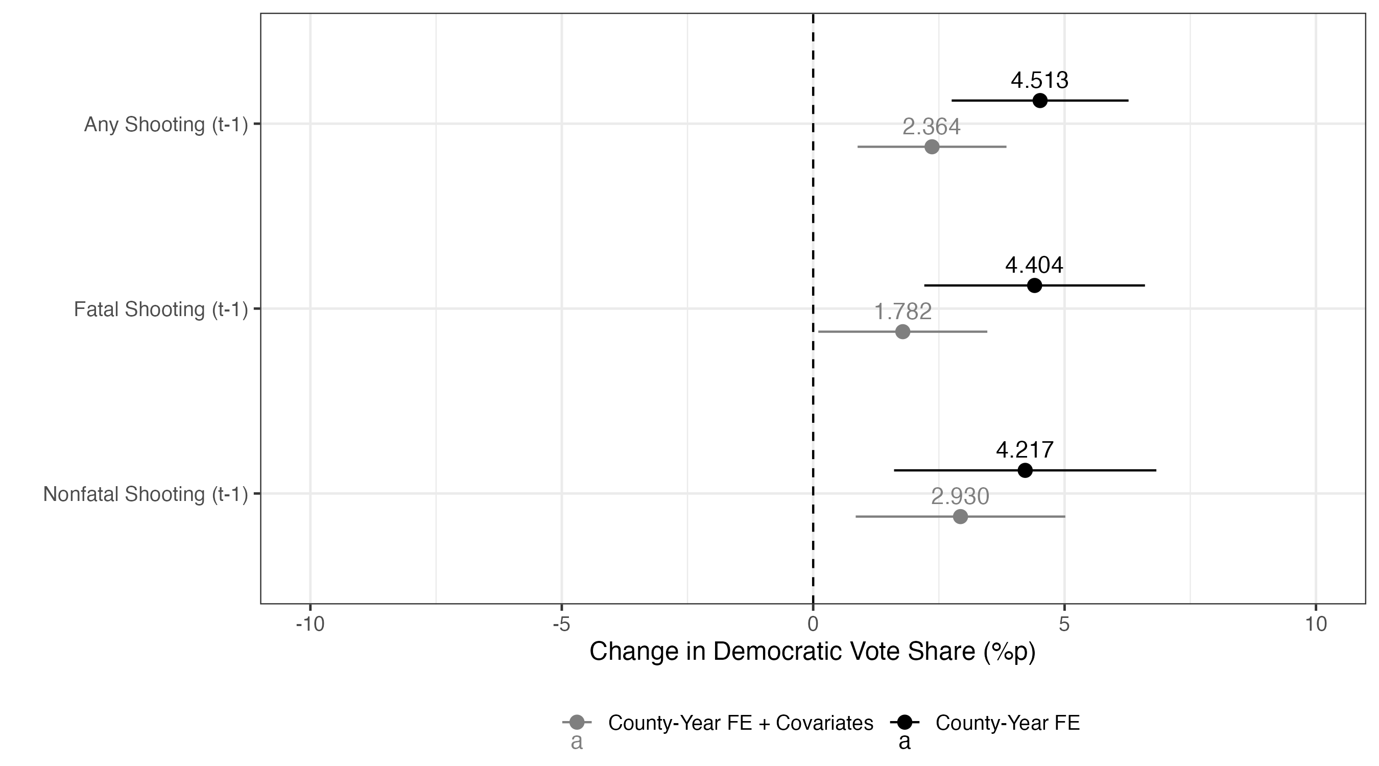
今回はいずれも統計的に有意な結果が得られている。例えば、モデル7(did_fit7)の場合、処置効果の推定値は4.513である。これは学校内銃撃事件が発生したカウンティーの場合、大統領選挙において民主党候補者の得票率が約4.513%p増加することを意味する。
以上の結果を図としてまとめてみよう。
<- tidy (did_fit7)<- tidy (did_fit8)<- tidy (did_fit9)<- tidy (did_fit10)<- tidy (did_fit11)<- tidy (did_fit12)<- bind_rows (list ("M1_Tr1" = tidy_fit7,"M2_Tr1" = tidy_fit8,"M1_Tr2" = tidy_fit9,"M2_Tr2" = tidy_fit10,"M1_Tr3" = tidy_fit11,"M2_Tr3" = tidy_fit12),.id = "Model" )
    Model               term      estimate    std.error statistic      p.value
1  M1_Tr1           shooting  4.513237e+00 8.752702e-01  5.156393 4.514820e-06
2  M2_Tr1           shooting  2.363839e+00 7.367346e-01  3.208536 2.353748e-03
3  M2_Tr1         population  3.174252e-05 6.778757e-06  4.682646 2.275534e-05
4  M2_Tr1          non_white  8.687344e+01 1.786287e+01  4.863352 1.234074e-05
5  M2_Tr1   change_unem_rate -1.389392e-01 1.274198e-01 -1.090405 2.808682e-01
6  M1_Tr2     fatal_shooting  4.404109e+00 1.091944e+00  4.033274 1.920110e-04
7  M2_Tr2     fatal_shooting  1.782393e+00 8.363792e-01  2.131083 3.812471e-02
8  M2_Tr2         population  3.206812e-05 6.801197e-06  4.715070 2.039958e-05
9  M2_Tr2          non_white  8.686629e+01 1.785535e+01  4.865000 1.227169e-05
10 M2_Tr2   change_unem_rate -1.392341e-01 1.275138e-01 -1.091914 2.802109e-01
11 M1_Tr3 non_fatal_shooting  4.216683e+00 1.298056e+00  3.248460 2.098382e-03
12 M2_Tr3 non_fatal_shooting  2.929866e+00 1.037217e+00  2.824737 6.825655e-03
13 M2_Tr3         population  3.229215e-05 6.717999e-06  4.806810 1.495567e-05
14 M2_Tr3          non_white  8.679618e+01 1.785514e+01  4.861131 1.243440e-05
15 M2_Tr3   change_unem_rate -1.400321e-01 1.274994e-01 -1.098296 2.774427e-01
        conf.low    conf.high df outcome
1   2.754316e+00 6.272159e+00 49 demvote
2   8.833157e-01 3.844363e+00 49 demvote
3   1.812010e-05 4.536494e-05 49 demvote
4   5.097665e+01 1.227702e+02 49 demvote
5  -3.949989e-01 1.171206e-01 49 demvote
6   2.209766e+00 6.598453e+00 49 demvote
7   1.016261e-01 3.463160e+00 49 demvote
8   1.840061e-05 4.573564e-05 49 demvote
9   5.098461e+01 1.227480e+02 49 demvote
10 -3.954828e-01 1.170146e-01 49 demvote
11  1.608142e+00 6.825225e+00 49 demvote
12  8.454996e-01 5.014232e+00 49 demvote
13  1.879182e-05 4.579247e-05 49 demvote
14  5.091493e+01 1.226774e+02 49 demvote
15 -3.962518e-01 1.161876e-01 49 demvote
<- did_est2 |> filter (grepl ("shooting" , term))
   Model               term estimate std.error statistic      p.value  conf.low
1 M1_Tr1           shooting 4.513237 0.8752702  5.156393 4.514820e-06 2.7543158
2 M2_Tr1           shooting 2.363839 0.7367346  3.208536 2.353748e-03 0.8833157
3 M1_Tr2     fatal_shooting 4.404109 1.0919440  4.033274 1.920110e-04 2.2097656
4 M2_Tr2     fatal_shooting 1.782393 0.8363792  2.131083 3.812471e-02 0.1016261
5 M1_Tr3 non_fatal_shooting 4.216683 1.2980560  3.248460 2.098382e-03 1.6081422
6 M2_Tr3 non_fatal_shooting 2.929866 1.0372173  2.824737 6.825655e-03 0.8454996
  conf.high df outcome
1  6.272159 49 demvote
2  3.844363 49 demvote
3  6.598453 49 demvote
4  3.463160 49 demvote
5  6.825225 49 demvote
6  5.014232 49 demvote
<- did_est2 |> separate (col = Model,into = c ("Model" , "Treat" ),sep = "_" )
  Model Treat               term estimate std.error statistic      p.value
1    M1   Tr1           shooting 4.513237 0.8752702  5.156393 4.514820e-06
2    M2   Tr1           shooting 2.363839 0.7367346  3.208536 2.353748e-03
3    M1   Tr2     fatal_shooting 4.404109 1.0919440  4.033274 1.920110e-04
4    M2   Tr2     fatal_shooting 1.782393 0.8363792  2.131083 3.812471e-02
5    M1   Tr3 non_fatal_shooting 4.216683 1.2980560  3.248460 2.098382e-03
6    M2   Tr3 non_fatal_shooting 2.929866 1.0372173  2.824737 6.825655e-03
   conf.low conf.high df outcome
1 2.7543158  6.272159 49 demvote
2 0.8833157  3.844363 49 demvote
3 2.2097656  6.598453 49 demvote
4 0.1016261  3.463160 49 demvote
5 1.6081422  6.825225 49 demvote
6 0.8454996  5.014232 49 demvote
<- did_est2 |> mutate (Model = if_else (Model == "M1" ,"County-Year FE" , "County-Year FE + Covariates" ),Treat = recode (Treat,"Tr1" = "Any Shooting (t-1)" ,"Tr2" = "Fatal Shooting (t-1)" ,"Tr3" = "Nonfatal Shooting (t-1)" ),Model = fct_rev (fct_inorder (Model)),Treat = fct_rev (fct_inorder (Treat)))
                        Model                   Treat               term
1              County-Year FE      Any Shooting (t-1)           shooting
2 County-Year FE + Covariates      Any Shooting (t-1)           shooting
3              County-Year FE    Fatal Shooting (t-1)     fatal_shooting
4 County-Year FE + Covariates    Fatal Shooting (t-1)     fatal_shooting
5              County-Year FE Nonfatal Shooting (t-1) non_fatal_shooting
6 County-Year FE + Covariates Nonfatal Shooting (t-1) non_fatal_shooting
  estimate std.error statistic      p.value  conf.low conf.high df outcome
1 4.513237 0.8752702  5.156393 4.514820e-06 2.7543158  6.272159 49 demvote
2 2.363839 0.7367346  3.208536 2.353748e-03 0.8833157  3.844363 49 demvote
3 4.404109 1.0919440  4.033274 1.920110e-04 2.2097656  6.598453 49 demvote
4 1.782393 0.8363792  2.131083 3.812471e-02 0.1016261  3.463160 49 demvote
5 4.216683 1.2980560  3.248460 2.098382e-03 1.6081422  6.825225 49 demvote
6 2.929866 1.0372173  2.824737 6.825655e-03 0.8454996  5.014232 49 demvote
|> ggplot () + geom_vline (xintercept = 0 , linetype = 2 ) + geom_pointrange (aes (x = estimate, xmin = conf.low, xmax = conf.high,y = Treat, color = Model),position = position_dodge2 (1 / 2 )) + geom_text (aes (x = estimate, y = Treat, color = Model, label = sprintf ("%.3f" , estimate)),position = position_dodge2 (1 / 2 ),vjust = - 0.75 ) + labs (x = "Change in Democratic Vote Share (%p)" , y = "" , color = "" ) + scale_color_manual (values = c ("County-Year FE" = "black" , "County-Year FE + Covariates" = "gray50" )) + coord_cartesian (xlim = c (- 10 , 10 )) + theme_bw (base_size = 12 ) + theme (legend.position = "bottom" )
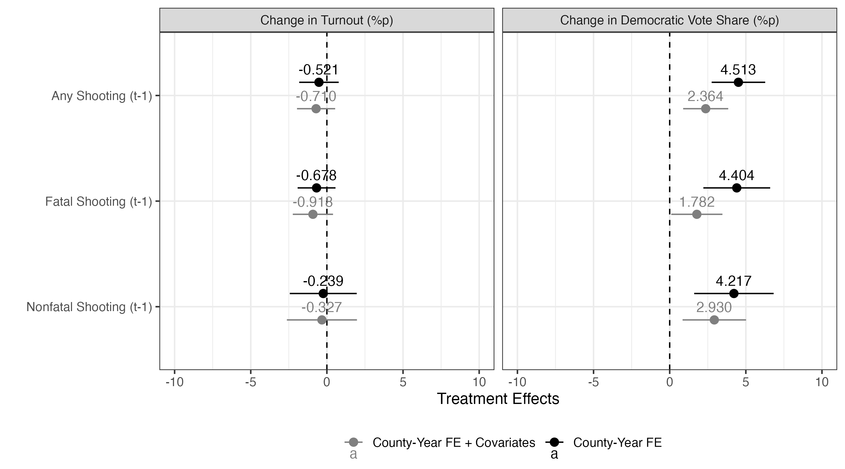
最後に、これまで作成した2つの図を一つにまとめてみよう。bind_rows()関数を使い、それぞれの表に識別子(Outcome)を与える。
<- bind_rows (list ("Out1" = did_est1,"Out2" = did_est2),.id = "Outcome" )
   Outcome                       Model                   Treat
1     Out1              County-Year FE      Any Shooting (t-1)
2     Out1 County-Year FE + Covariates      Any Shooting (t-1)
3     Out1              County-Year FE    Fatal Shooting (t-1)
4     Out1 County-Year FE + Covariates    Fatal Shooting (t-1)
5     Out1              County-Year FE Nonfatal Shooting (t-1)
6     Out1 County-Year FE + Covariates Nonfatal Shooting (t-1)
7     Out2              County-Year FE      Any Shooting (t-1)
8     Out2 County-Year FE + Covariates      Any Shooting (t-1)
9     Out2              County-Year FE    Fatal Shooting (t-1)
10    Out2 County-Year FE + Covariates    Fatal Shooting (t-1)
11    Out2              County-Year FE Nonfatal Shooting (t-1)
12    Out2 County-Year FE + Covariates Nonfatal Shooting (t-1)
                 term   estimate std.error  statistic      p.value   conf.low
1            shooting -0.5210841 0.6456718 -0.8070417 4.235426e-01 -1.8186103
2            shooting -0.7097922 0.6237320 -1.1379763 2.606641e-01 -1.9632286
3      fatal_shooting -0.6779229 0.6191749 -1.0948810 2.789215e-01 -1.9222015
4      fatal_shooting -0.9179995 0.6576559 -1.3958659 1.690478e-01 -2.2396086
5  non_fatal_shooting -0.2387205 1.0938325 -0.2182423 8.281467e-01 -2.4368592
6  non_fatal_shooting -0.3269742 1.1453027 -0.2854915 7.764710e-01 -2.6285461
7            shooting  4.5132372 0.8752702  5.1563930 4.514820e-06  2.7543158
8            shooting  2.3638394 0.7367346  3.2085357 2.353748e-03  0.8833157
9      fatal_shooting  4.4041092 1.0919440  4.0332738 1.920110e-04  2.2097656
10     fatal_shooting  1.7823931 0.8363792  2.1310825 3.812471e-02  0.1016261
11 non_fatal_shooting  4.2166835 1.2980560  3.2484602 2.098382e-03  1.6081422
12 non_fatal_shooting  2.9298657 1.0372173  2.8247368 6.825655e-03  0.8454996
   conf.high df outcome
1  0.7764420 49 turnout
2  0.5436442 49 turnout
3  0.5663557 49 turnout
4  0.4036096 49 turnout
5  1.9594182 49 turnout
6  1.9745977 49 turnout
7  6.2721585 49 demvote
8  3.8443631 49 demvote
9  6.5984529 49 demvote
10 3.4631600 49 demvote
11 6.8252248 49 demvote
12 5.0142319 49 demvote
Outcome列のリコーディングし、factor化する。
<- did_est |> mutate (Outcome = if_else (Outcome == "Out1" ,"Change in Turnout (%p)" ,"Change in Democratic Vote Share (%p)" ),Outcome = fct_inorder (Outcome))
                                Outcome                       Model
1                Change in Turnout (%p)              County-Year FE
2                Change in Turnout (%p) County-Year FE + Covariates
3                Change in Turnout (%p)              County-Year FE
4                Change in Turnout (%p) County-Year FE + Covariates
5                Change in Turnout (%p)              County-Year FE
6                Change in Turnout (%p) County-Year FE + Covariates
7  Change in Democratic Vote Share (%p)              County-Year FE
8  Change in Democratic Vote Share (%p) County-Year FE + Covariates
9  Change in Democratic Vote Share (%p)              County-Year FE
10 Change in Democratic Vote Share (%p) County-Year FE + Covariates
11 Change in Democratic Vote Share (%p)              County-Year FE
12 Change in Democratic Vote Share (%p) County-Year FE + Covariates
                     Treat               term   estimate std.error  statistic
1       Any Shooting (t-1)           shooting -0.5210841 0.6456718 -0.8070417
2       Any Shooting (t-1)           shooting -0.7097922 0.6237320 -1.1379763
3     Fatal Shooting (t-1)     fatal_shooting -0.6779229 0.6191749 -1.0948810
4     Fatal Shooting (t-1)     fatal_shooting -0.9179995 0.6576559 -1.3958659
5  Nonfatal Shooting (t-1) non_fatal_shooting -0.2387205 1.0938325 -0.2182423
6  Nonfatal Shooting (t-1) non_fatal_shooting -0.3269742 1.1453027 -0.2854915
7       Any Shooting (t-1)           shooting  4.5132372 0.8752702  5.1563930
8       Any Shooting (t-1)           shooting  2.3638394 0.7367346  3.2085357
9     Fatal Shooting (t-1)     fatal_shooting  4.4041092 1.0919440  4.0332738
10    Fatal Shooting (t-1)     fatal_shooting  1.7823931 0.8363792  2.1310825
11 Nonfatal Shooting (t-1) non_fatal_shooting  4.2166835 1.2980560  3.2484602
12 Nonfatal Shooting (t-1) non_fatal_shooting  2.9298657 1.0372173  2.8247368
        p.value   conf.low conf.high df outcome
1  4.235426e-01 -1.8186103 0.7764420 49 turnout
2  2.606641e-01 -1.9632286 0.5436442 49 turnout
3  2.789215e-01 -1.9222015 0.5663557 49 turnout
4  1.690478e-01 -2.2396086 0.4036096 49 turnout
5  8.281467e-01 -2.4368592 1.9594182 49 turnout
6  7.764710e-01 -2.6285461 1.9745977 49 turnout
7  4.514820e-06  2.7543158 6.2721585 49 demvote
8  2.353748e-03  0.8833157 3.8443631 49 demvote
9  1.920110e-04  2.2097656 6.5984529 49 demvote
10 3.812471e-02  0.1016261 3.4631600 49 demvote
11 2.098382e-03  1.6081422 6.8252248 49 demvote
12 6.825655e-03  0.8454996 5.0142319 49 demvote
図の作り方はこれまでと変わらないが、ファセット分割を行うため、facet_wrap()レイヤーを追加する。
|> ggplot () + geom_vline (xintercept = 0 , linetype = 2 ) + geom_pointrange (aes (x = estimate, xmin = conf.low, xmax = conf.high,y = Treat, color = Model),position = position_dodge2 (1 / 2 )) + geom_text (aes (x = estimate, y = Treat, color = Model, label = sprintf ("%.3f" , estimate)),position = position_dodge2 (1 / 2 ),vjust = - 0.75 ) + labs (x = "Treatment Effects" , y = "" , color = "" ) + scale_color_manual (values = c ("County-Year FE" = "black" , "County-Year FE + Covariates" = "gray50" )) + coord_cartesian (xlim = c (- 10 , 10 )) + facet_wrap (~ Outcome, ncol = 2 ) + theme_bw (base_size = 12 ) + theme (legend.position = "bottom" )
以上の結果から「学校内銃撃事件の発生は投票参加を促すとは言えないものの、民主党候補者の得票率を上げる」ということが言えよう。