マクロ政治データ分析実習
9/ 分析結果の報告
参考)回帰表の可視化
{modelsummary}のmodelplot()関数
modelplot()から作成された図は{ggplot2}ベースなので+でレイヤーの追加、調整が可能- 詳細は
?modelplotか公式ページで確認すること。他にも{coefplot}も人気(存在感のない{coefplotbl}というのもある)
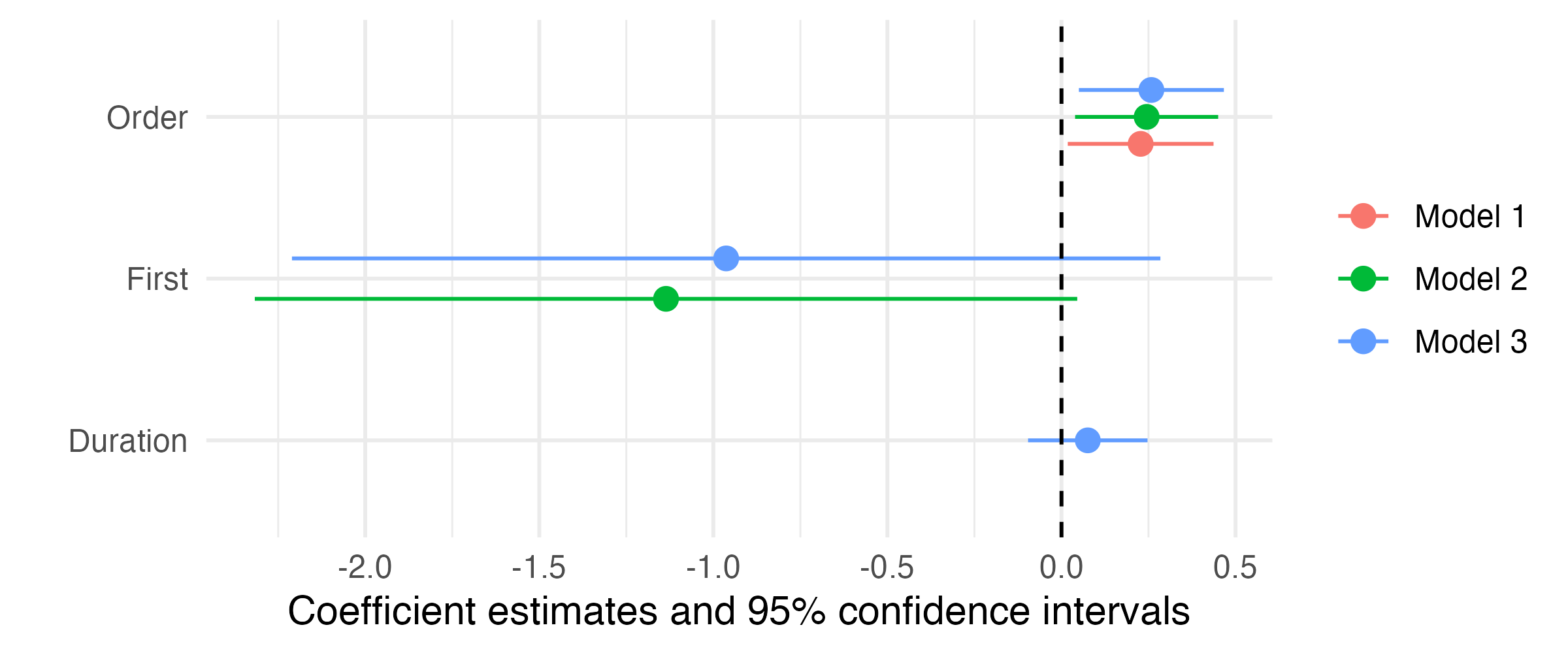
作図の例
Pointrangeプロットを使用する。
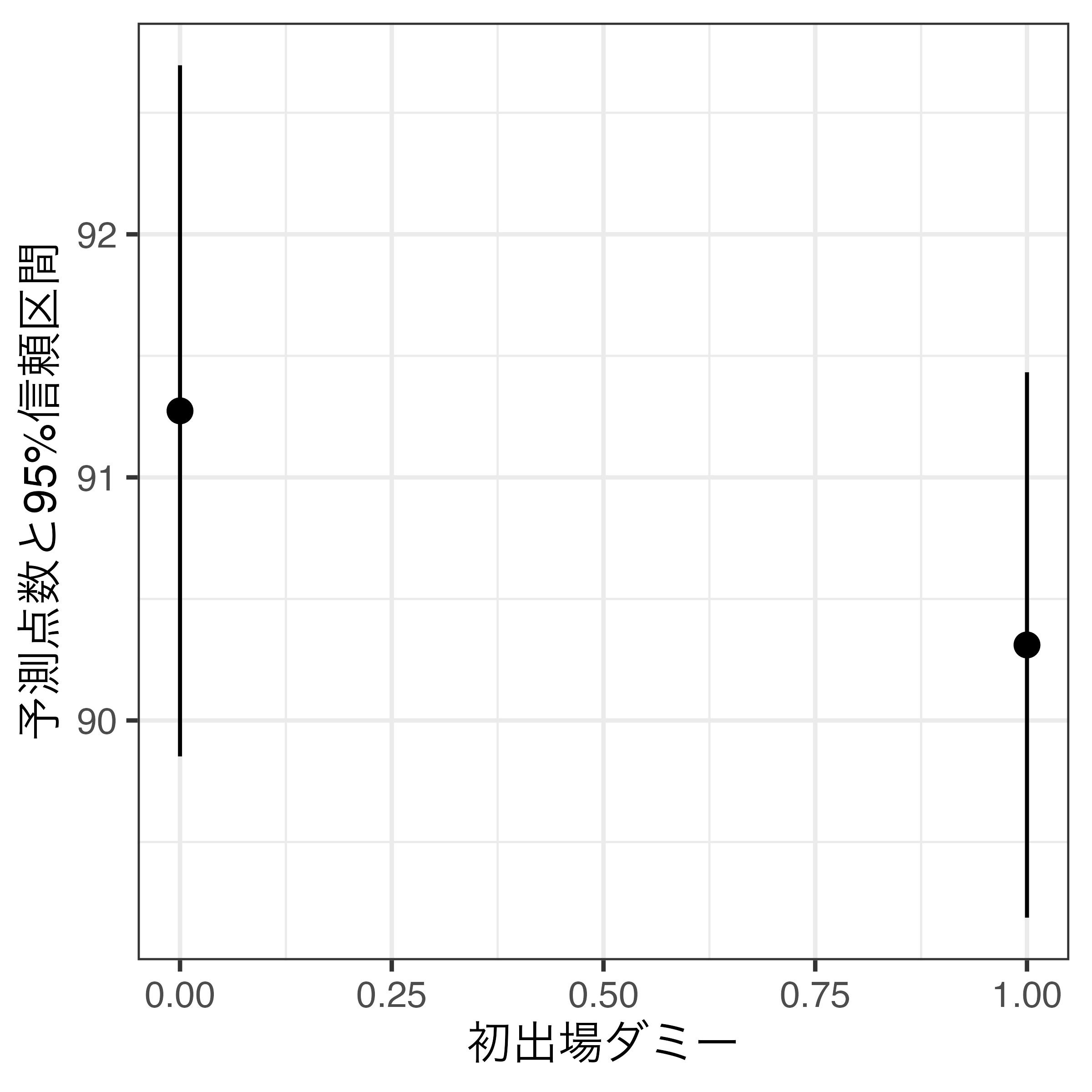
無駄の目盛りの削除
- 横軸(X軸)の無駄な目盛りを削除し、0と1のみ残す。

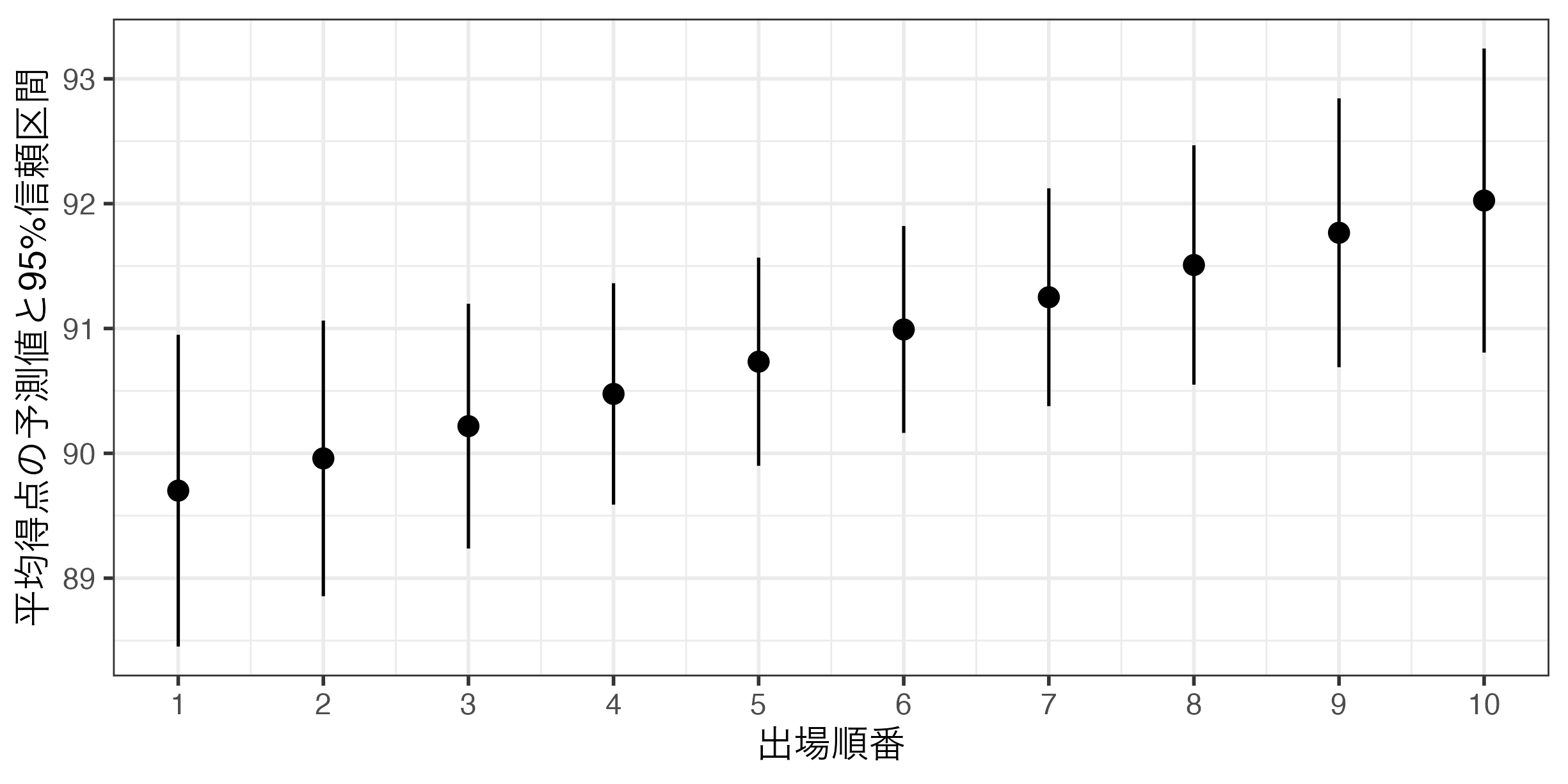
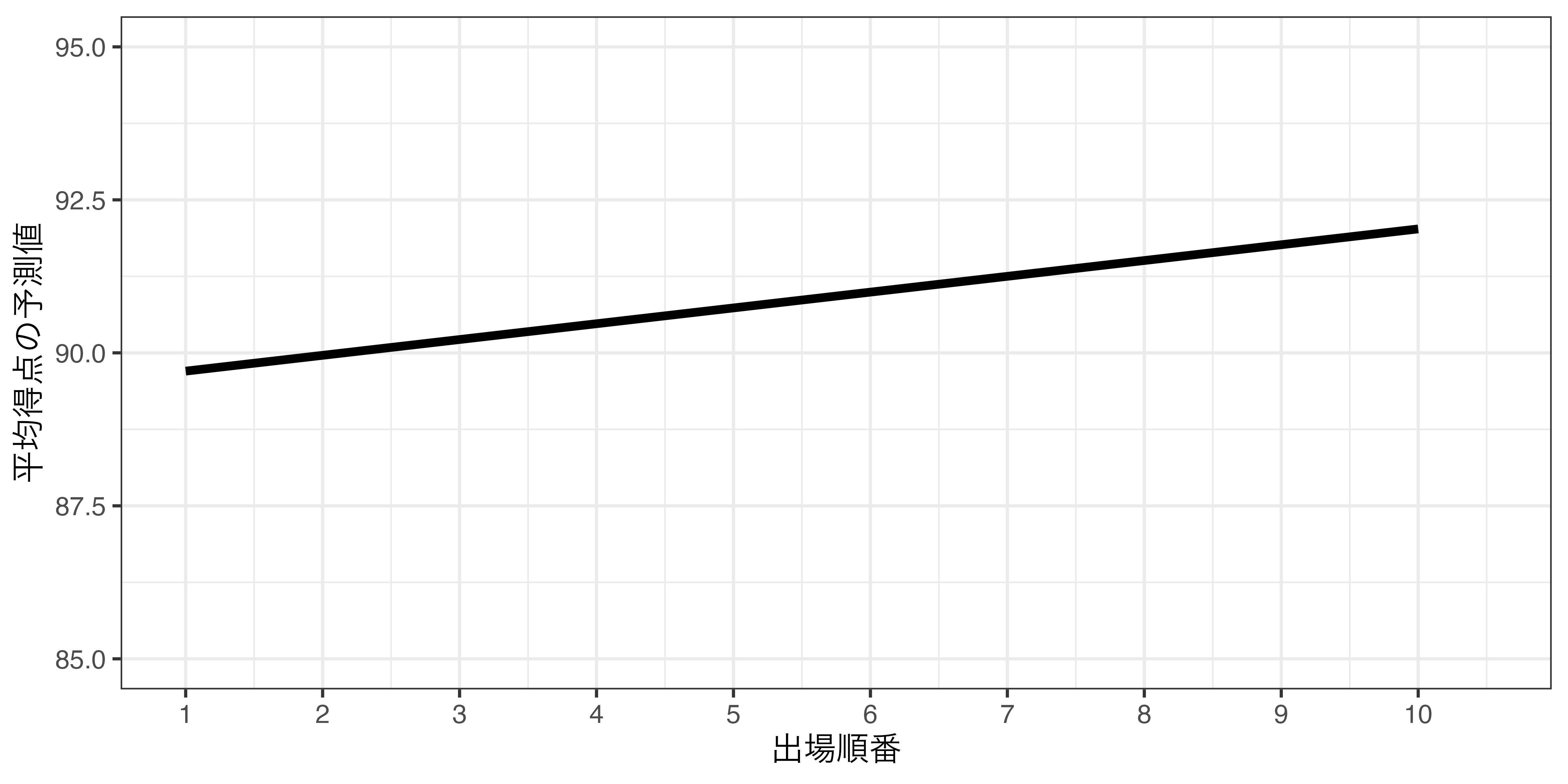
出場順番と平均得点間の関係(可視化)
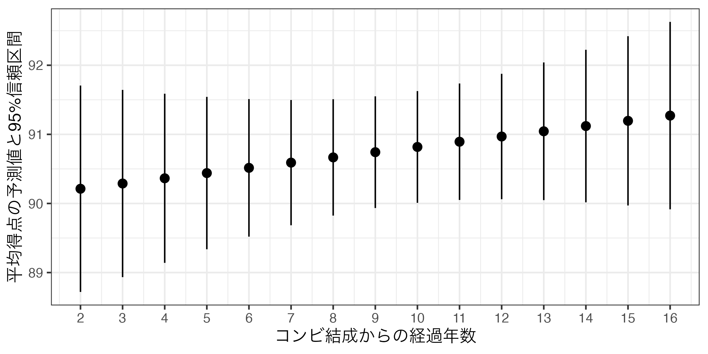
芸歴と平均得点間の関係(可視化)
折れ線グラフとリボン(geom_ribbon())の組み合わせ
- 横軸が細かいほどpoint-rangeプロットは気持ち悪くなる(ムカデのような見た目になる)。
geom_ribbon()はx、ymin、ymaxにマッピングgeom_pointrange()と使い方は同じだが、予測値の情報を持たないため、yは不要
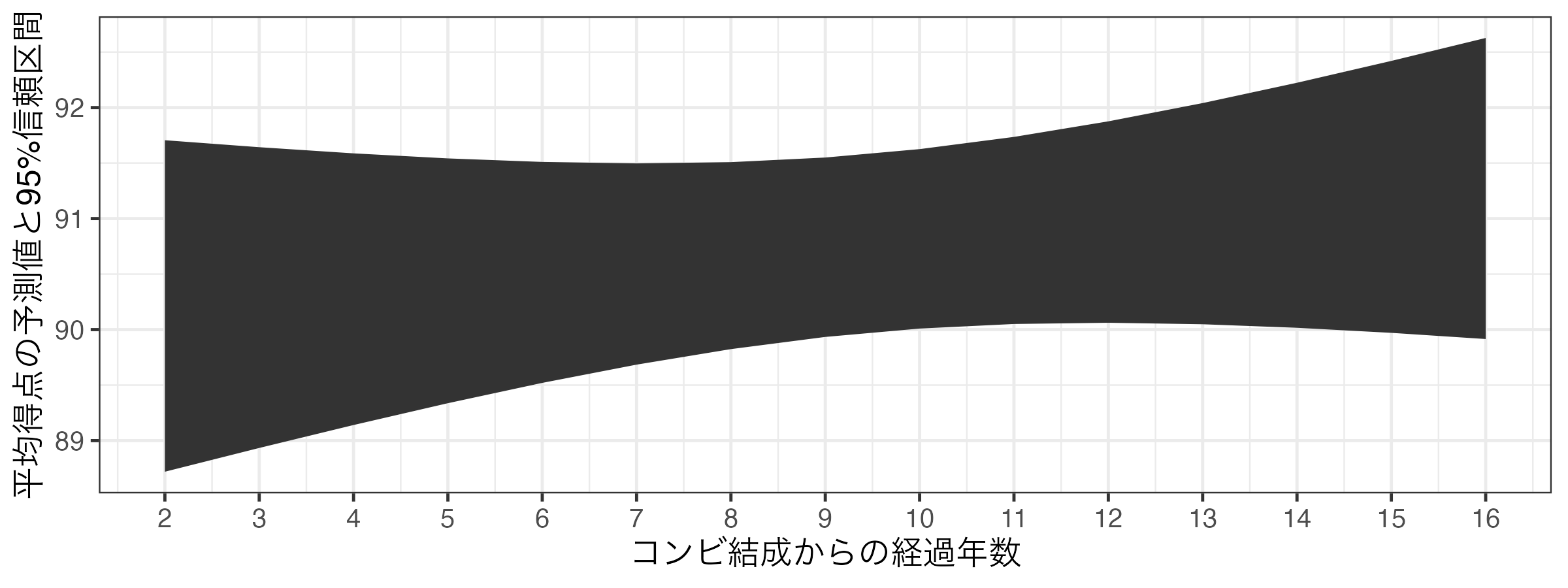
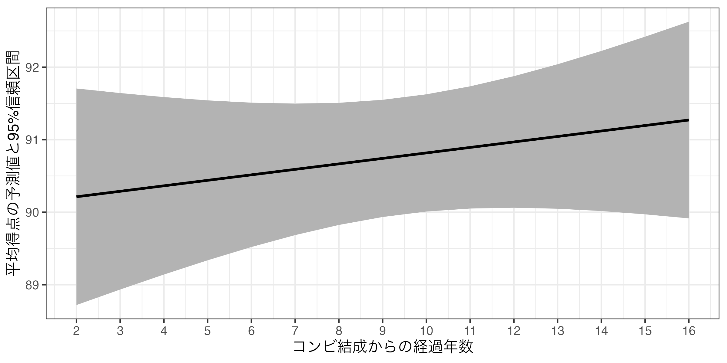
折れ線グラフ + リボン
- 1
-
geom_ribbon()とgeom_line()は同じ横軸を共有するため、ここでマッピングした方が効率的 - 2
- デフォルトのリボンは暗い色なので、明るめの色に変える。
- 3
-
linewidthで折れ線グラフの太さを調整(1だとデフォルトよりやや太め)
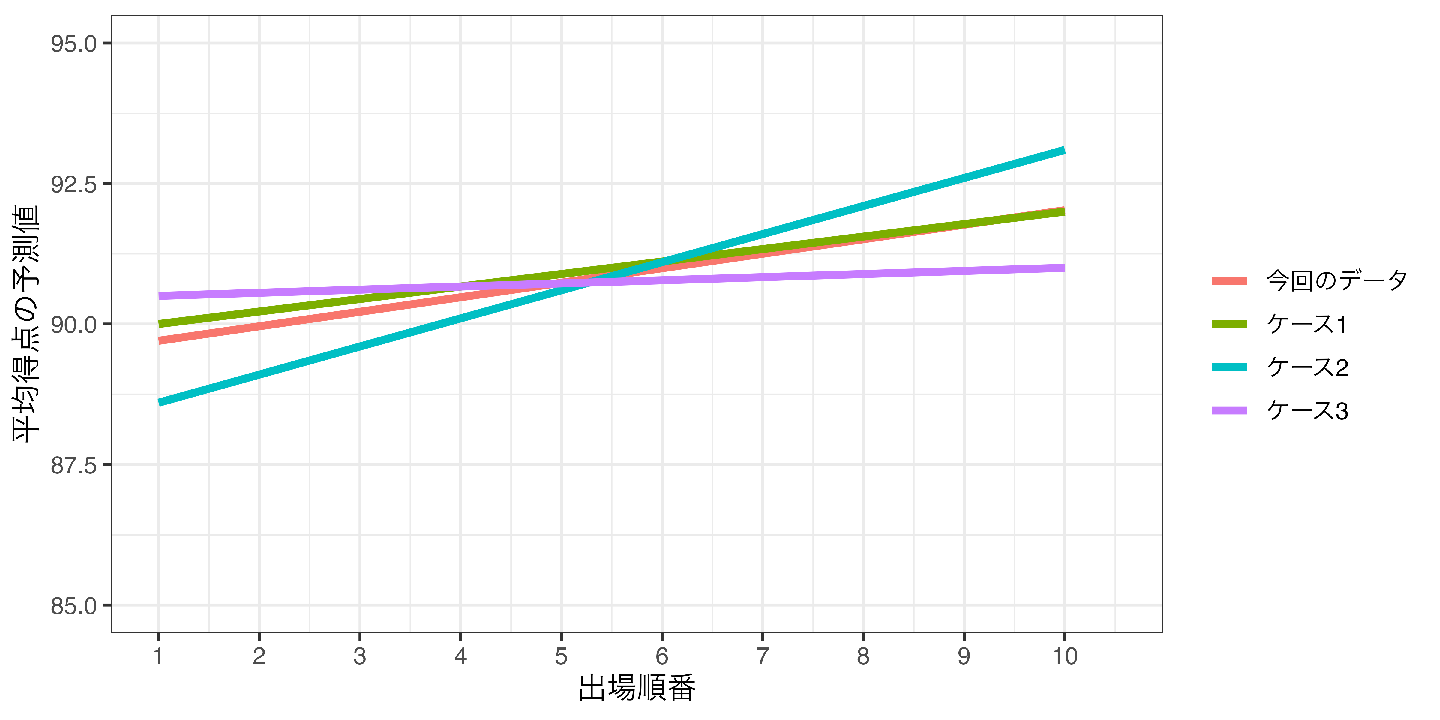
出場順番と平均得点間の関係
今回得られた回帰直線
もう一度、過去に戻ってM-1をやったら…(1)
こんな回帰直線が得られたとしてもおかしくはない(多分)
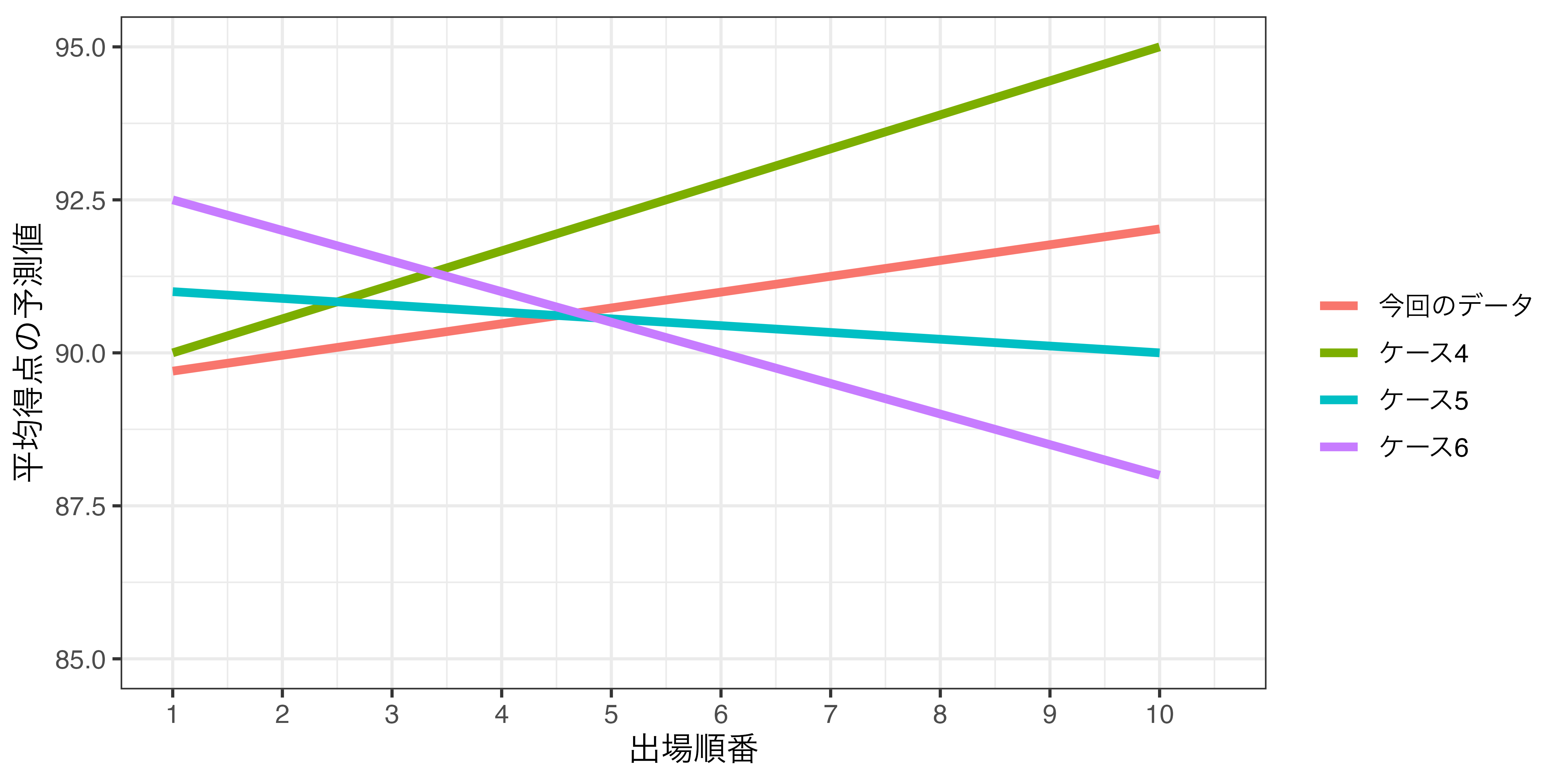
もう一度、過去に戻ってM-1をやったら…(2)
こんな回帰直線が得られる可能性は非常に低い(多分)
信頼区間の意味
この範囲(信頼区間)外の直線が得られる可能性は非常に低い!
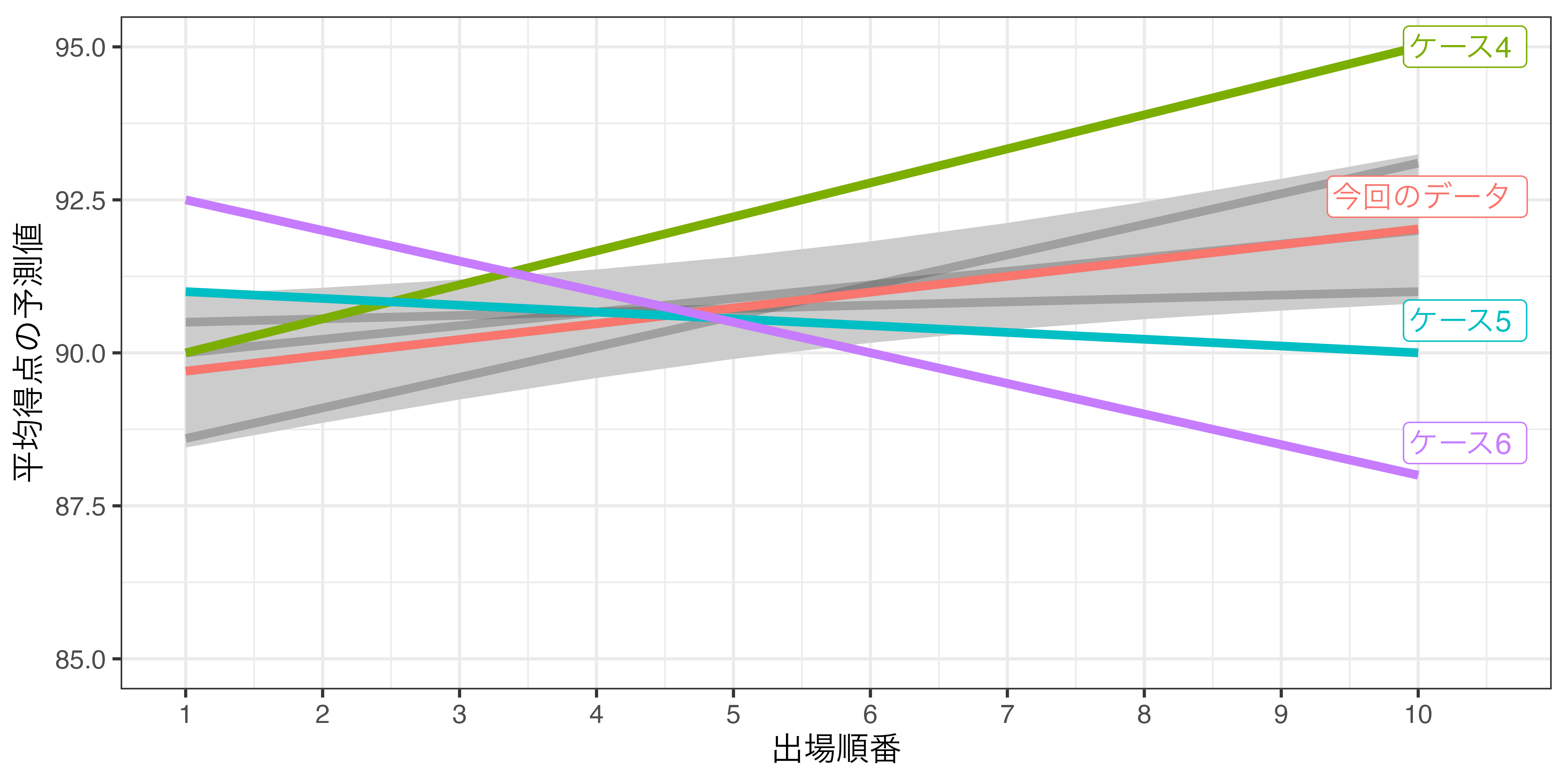
信頼区間の意味(2)
傾き係数が正(負)に統計的有意であれば、この区間内に引ける直線は必ず右上がり(右下がり)となる。
- \(\alpha\) = 0.05で統計的有意だった
Order(\(p\) = 0.016)は、95%信頼区間内に右上がりの直線しか引けない。 - 右は統計的に有意でない
Duration変数の例(\(p\) = 0.381)- 水平線も、右上がり直線も、右下がり直線も引ける。
- \(\Rightarrow\)
DurationとScore_Meanの関係(正か負)は現段階では判断できない。
- \(\alpha\) = 0.1を仮定するのであれば、90%(\(= (1 - \alpha) \times 100\))信頼区間を使うこととなる。
有意水準と信頼区間
\(\alpha\) = 0.6を採用する場合、40%信頼区間(\((1 - \alpha) \times 100\)%信頼区間)を使うと…
- 以下は40%信頼区間を採用した例(
predictions()内にconf_level = 0.4を追加する)- ただし、よく使うのは90%(\(\alpha\) = 0.1)、95%(\(\alpha\) = 0.05)、99%(\(\alpha\) = 0.01)信頼区間
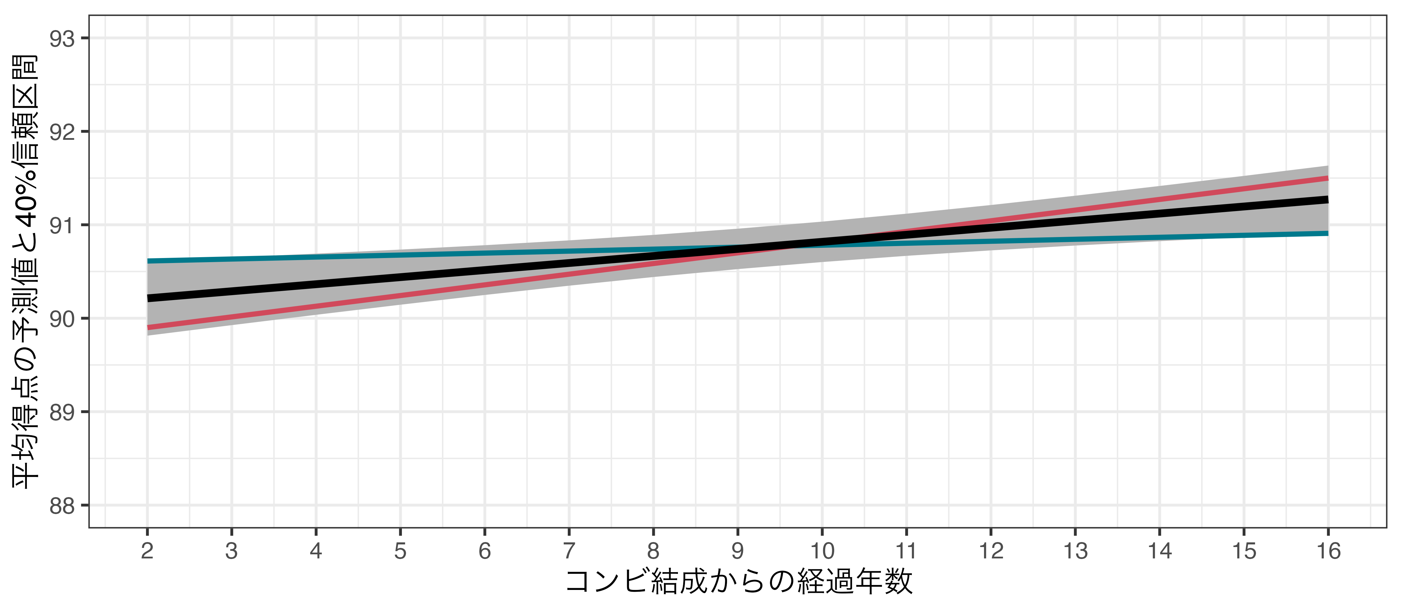
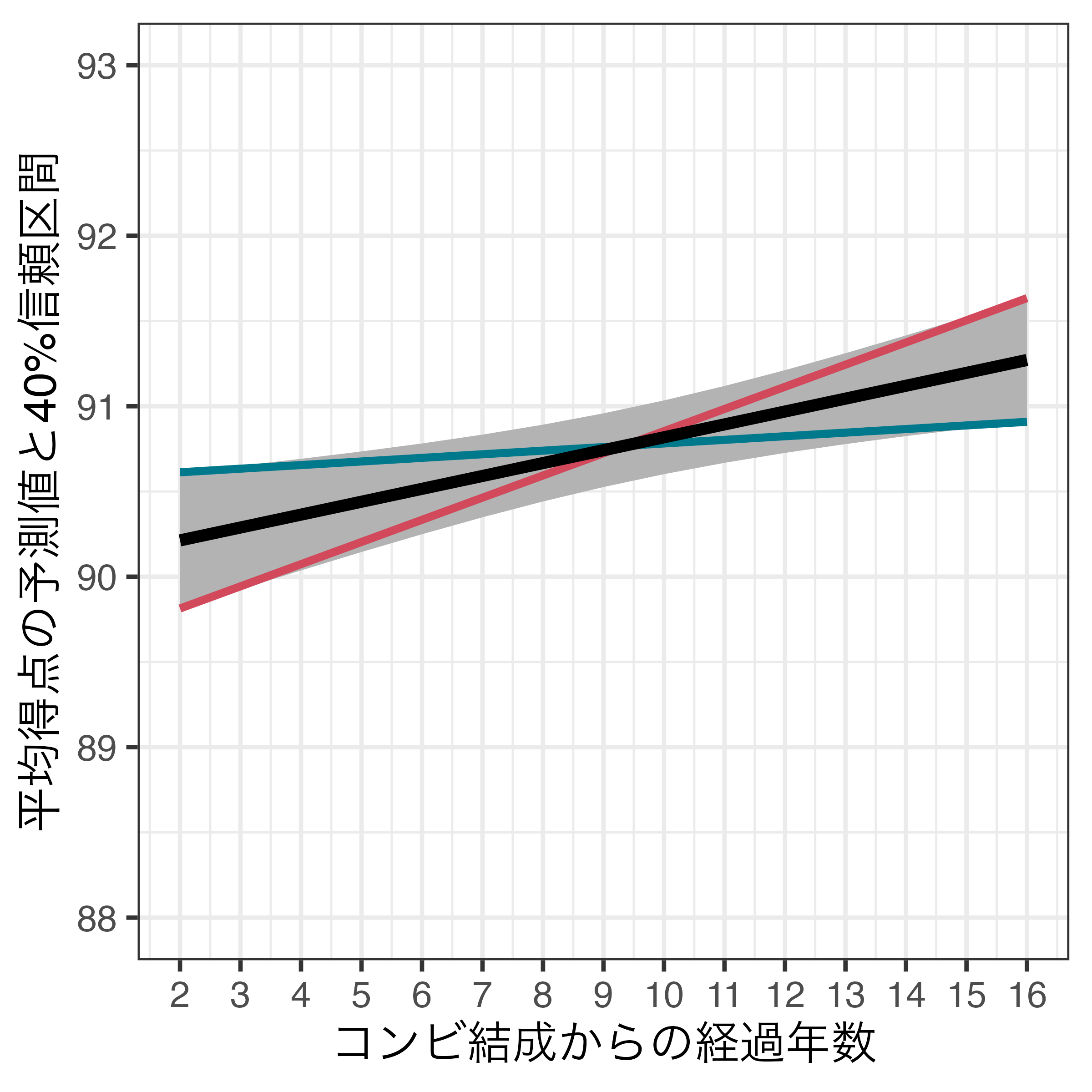
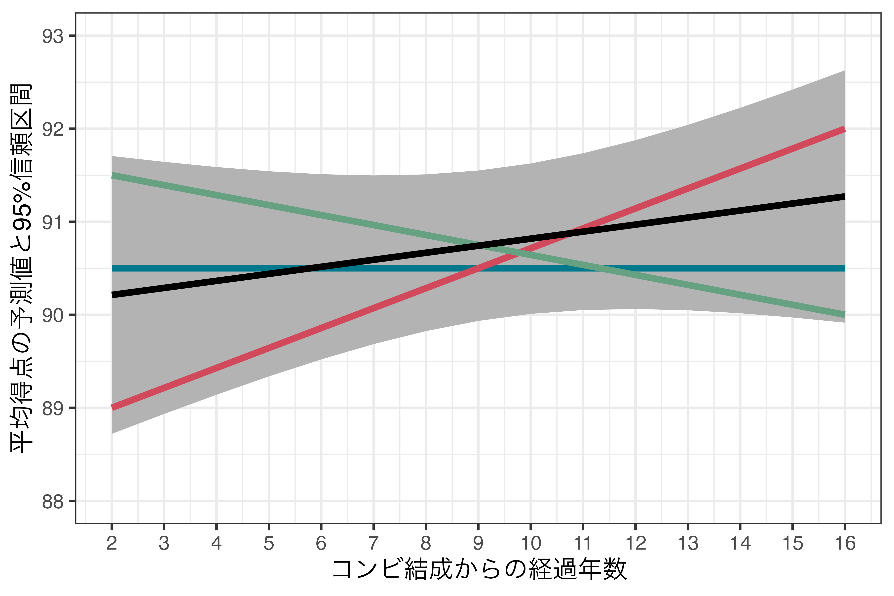
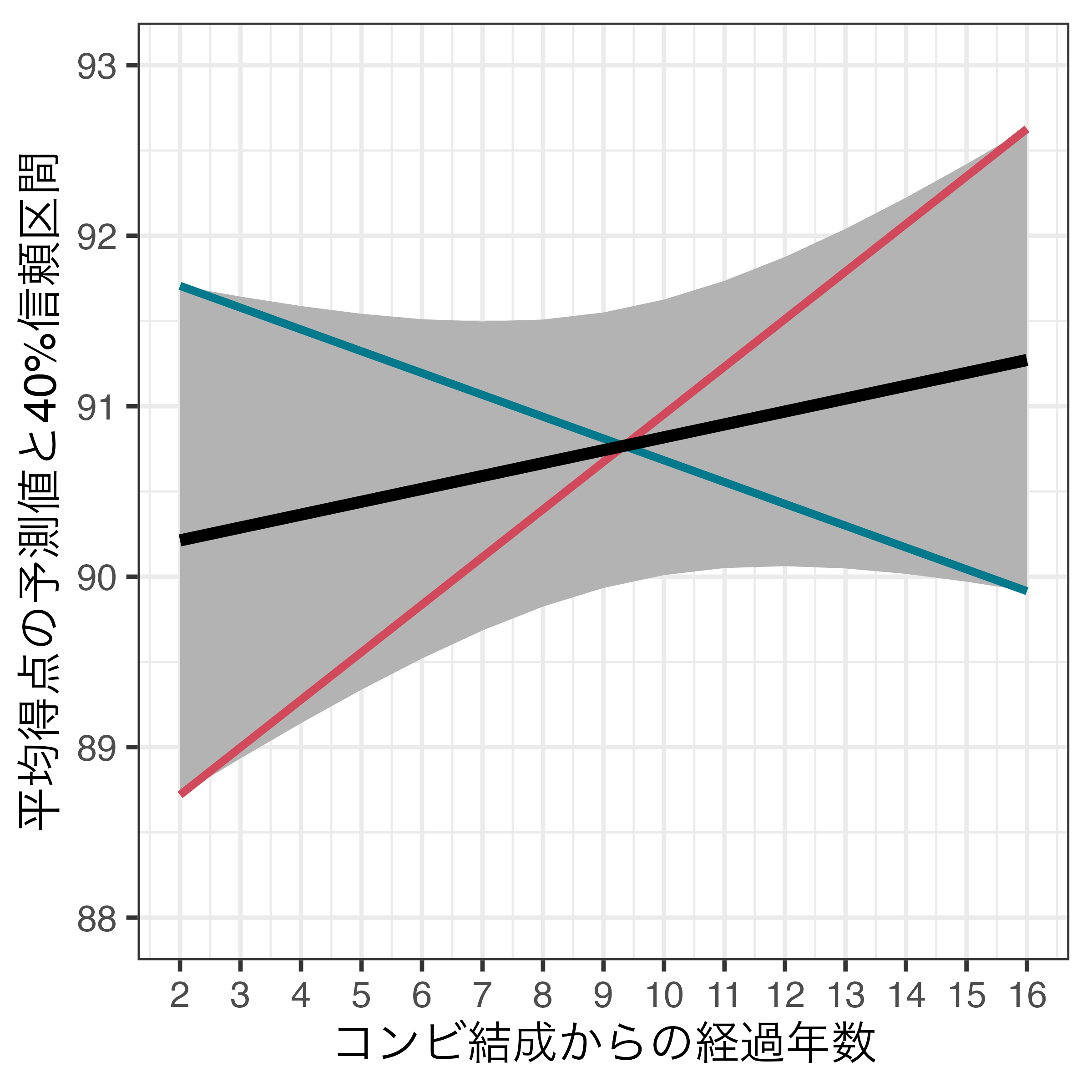
95%信頼区間と40%信頼区間の比較
- 青線
- 左端の座標:\((x = 2, y = 91.706)\)
- 右端の座標:\((x = 16, y = 89.916)\)
- \(\Rightarrow\) 右下がり
- 赤線
- 左端の座標:\((x = 2, y = 88.720)\)
- 右端の座標:\((x = 16, y = 92.627)\)
- \(\Rightarrow\) 右上がり
- \(\Rightarrow\) 右上がり、右下がりの直線が入り得るため、\(\alpha = 0.05\)の場合、「コンビ結成からの経過年数」と「平均得点」間の統計的に有意な関係は見られない。
- 青線
- 左端の座標:\((x = 2, y = 90.612)\)
- 右端の座標:\((x = 16, y = 90.808)\)
- \(\Rightarrow\) 右上がり
- 赤線
- 左端の座標:\((x = 2, y = 89.813)\)
- 右端の座標:\((x = 16, y = 91.634)\)
- \(\Rightarrow\) 右上がり
- \(\Rightarrow\) 右上がりの直線しか入らないため、\(\alpha = 0.6\)の場合、「コンビ結成からの経過年数」と「平均得点」間の統計的に有意な正の関係が見られる。