社会科学における因果推論

3/ 無作為化比較試験

宋(そん)  財泫(じぇひょん)

関西大学総合情報学部

信頼できるATEの条件

内生性の存在 \(\rightarrow\) ATE推定値の信頼性\(\downarrow\)

例) やる気のある学生だけがソンさんの講義を履修した場合

1. 自己選択バイアス
   • ソンさんの講義は鬼畜すぎるため、やる気満々の学生には役に立つものの、やる気のない学生にとってはむしろ学習意欲が低下
2. 疑似相関
   • やる気のある学生はいろんな方面で頑張るから、将来年収が高くなる。
3. 測定誤差
   • 履修者の年収はジンバブエ・ドルで測定されている可能性も（これはないか）

内生性は因果推論の敵! どうすれば…?

\(\downarrow\)

無作為割当 (Random Assignment)

無作為割当とは

無作為割当 (Random Assignment)

• 処置を受けるかどうかを無作為に割り当てる方法
  • 完全無作為割当: 全ての被験者において、どのグループに属するかの確率が等しい
  • \(Pr(T_i = 1) = Pr(T_j = 1) \text{ where } i \neq j\)
  • \(Pr(T_i = 0) = Pr(T_j = 0) \text{ where } i \neq j\)
  • 無作為割当の方法は色々
• 無作為に割り当てると、処置を受けないグループと処置を受けるグループは「集団」として同質なグループになる。
  • 受けないグループ: 統制群 (Control Group)
  • 受けるグループ: 処置群 (Treatment Group)
• 一つの集団を一人の個人として扱い、ITEを測定 ⇒ ATE

無作為割当の力

コインを投げ、表( \(H\) )なら統制群、裏( \(T\) )なら処置群に割当

• データ生成
• Dataの中身

set.seed(19861008)
Data <- tibble(ID = 1:20,
               Female = sample(0:1, 20, replace = TRUE, 
                               prob = c(0.4, 0.6)),
               Age    = round(rnorm(20, 38, 10), 0))

Data |>
   summarise(Female = mean(Female),
             Age    = mean(Age))

# A tibble: 1 × 2
  Female   Age
   <dbl> <dbl>
1   0.55    38

ID	Female	Age		ID	Female	Age
1	1	31		11	0	38
2	1	41		12	1	29
3	0	31		13	0	21
4	1	46		14	0	26
5	1	37		15	1	36
6	1	37		16	1	40
7	0	30		17	0	50
8	1	46		18	0	42
9	1	56		19	0	29
10	0	47		20	1	47

無作為割当の力

コイン投げの結果

• コイン投げ
• Dataの中身

set.seed(19861008)
Coin <- sample(c("H", "T"), 20, replace = TRUE)
Coin

 [1] "H" "T" "T" "T" "H" "H" "H" "T" "H" "H" "H" "T" "H" "T" "H" "T" "T" "T" "H"
[20] "H"

table(Coin)

Coin
 H  T 
11  9 

Data$Coin <- Coin

ID	Female	Age	Coin		ID	Female	Age	Coin
1	1	31	H		11	0	38	H
2	1	41	T		12	1	29	T
3	0	31	T		13	0	21	H
4	1	46	T		14	0	26	T
5	1	37	H		15	1	36	H
6	1	37	H		16	1	40	T
7	0	30	H		17	0	50	T
8	1	46	T		18	0	42	T
9	1	56	H		19	0	29	H
10	0	47	H		20	1	47	H

無作為割当の力

統制群と処置群が比較的同質的なグループに

• 統制群（11名）: 女性比率が54.5%、平均年齢が37.2歳
• 処置群 (9名): 女性比率が55.6%、平均年齢が39歳

Data |>
  group_by(Coin) |>
  summarise(Female = mean(Female),
            Age    = mean(Age),
            N      = n())

# A tibble: 2 × 4
  Coin  Female   Age     N
  <chr>  <dbl> <dbl> <int>
1 H      0.545  37.2    11
2 T      0.556  39       9

無作為割当の力

集団として処置群と統制群は、母集団とほぼ同質

• \(n \rightarrow \infty\) なら2つのグループはより同質的に（大数の弱法則）

	女性の割合	平均年齢
母集団（\(n=20\)）	55.0%	38.0歳
統制群（\(n=11\)）	54.5%	37.2歳
処置群（\(n=9\)）	55.6%	39.0歳

• 統制群と処置群、母集団はそれぞれ交換可能（exchangeable）
  • 処置群に処置を与えること = 母集団全体に処置を与えること
  • 統制群に処置を与えないこと = 母集団全体に処置を与えないこと
• 統制群と処置群の比較で集団を一つの単位としたITE（= ATE）が推定可能
  • 処置を与えた母集団 vs. 処置を与えなかった母集団

無作為割当の力

無作為割当は均質な複数のグループを作る手法

• 講義履修と年収の例だと、無作為割当をすることによって …
  • 各グループにやる気のある学生とない学生が均等に
    • 自己選択バイアス、擬似相関の除去
  • ジンバブエ・ドルで測定される学生も均等に（これはないか）
    • 測定誤差の除去
• 内生性:処置変数（講義の履修）と誤差項（やる気など）間の相関
  • コイン投げの結果は被験者（学生）の性質と無関係に行われるため、誤差項と相関がない。
  • 外生変数（Exogenous variable）
  • 学生の性質（\(X\)）と処置有無（\(T\)）は独立している ⇒ \(X \perp T\)

無作為割当は内生性を除去する最良の手法

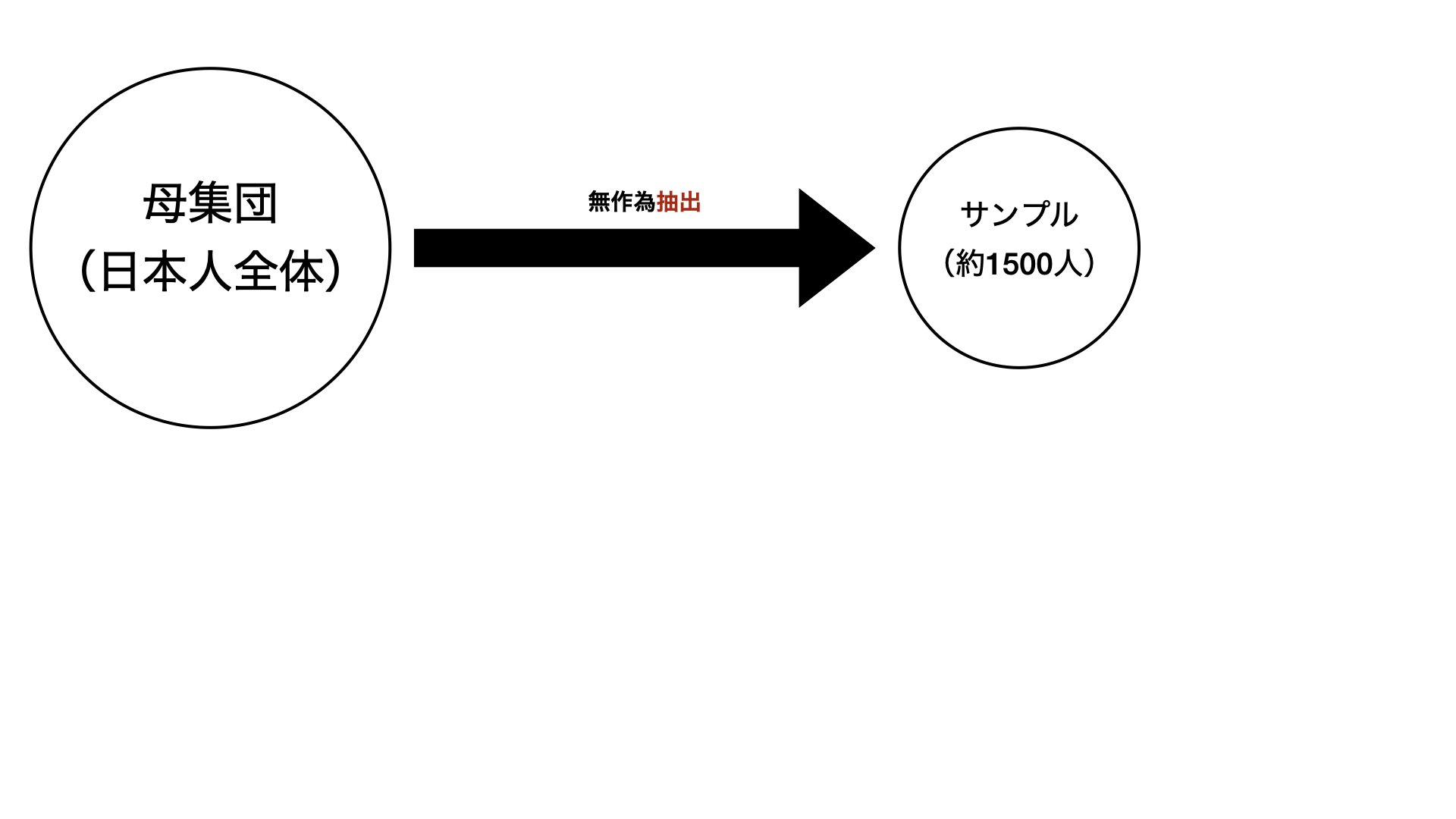
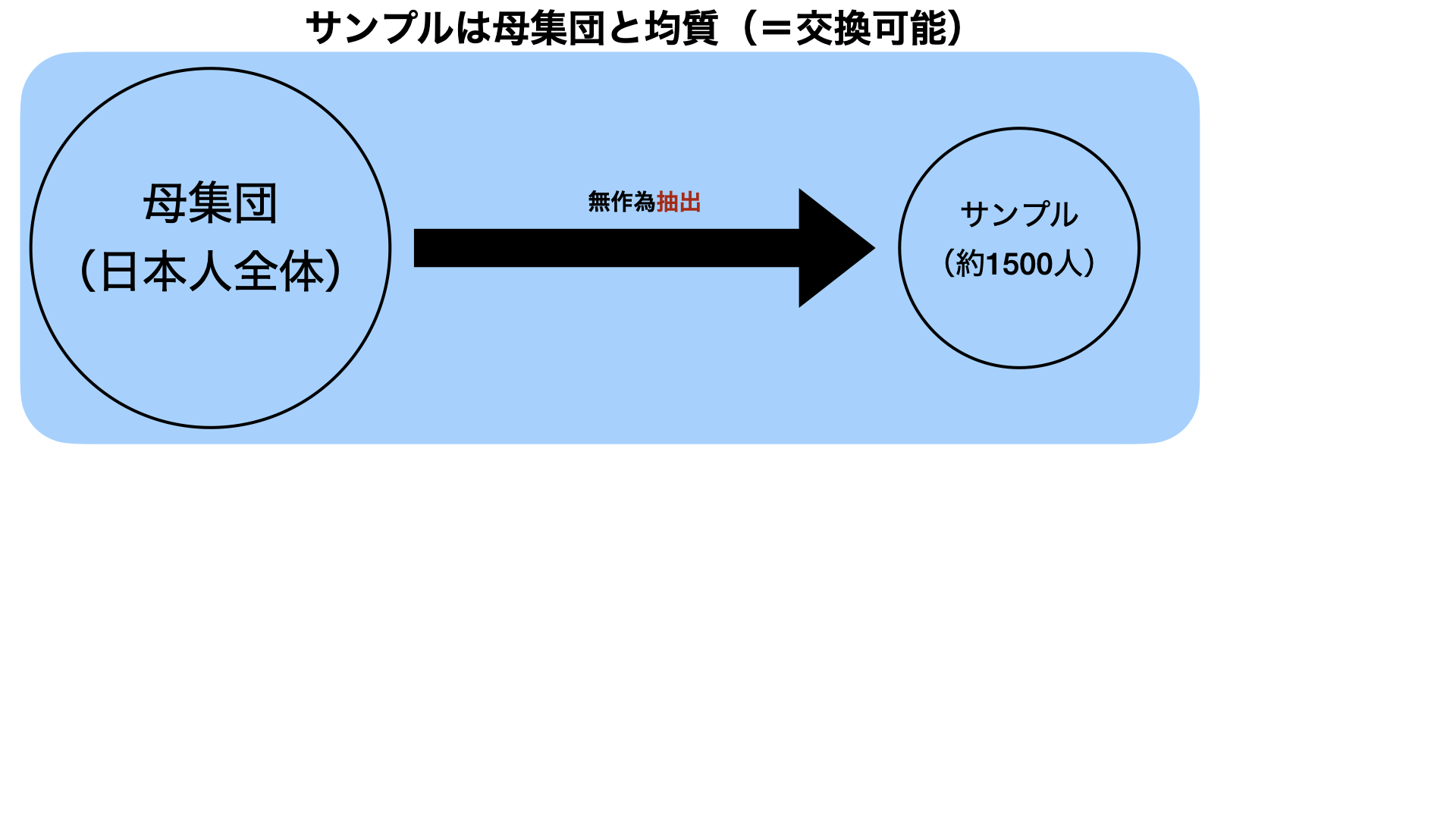
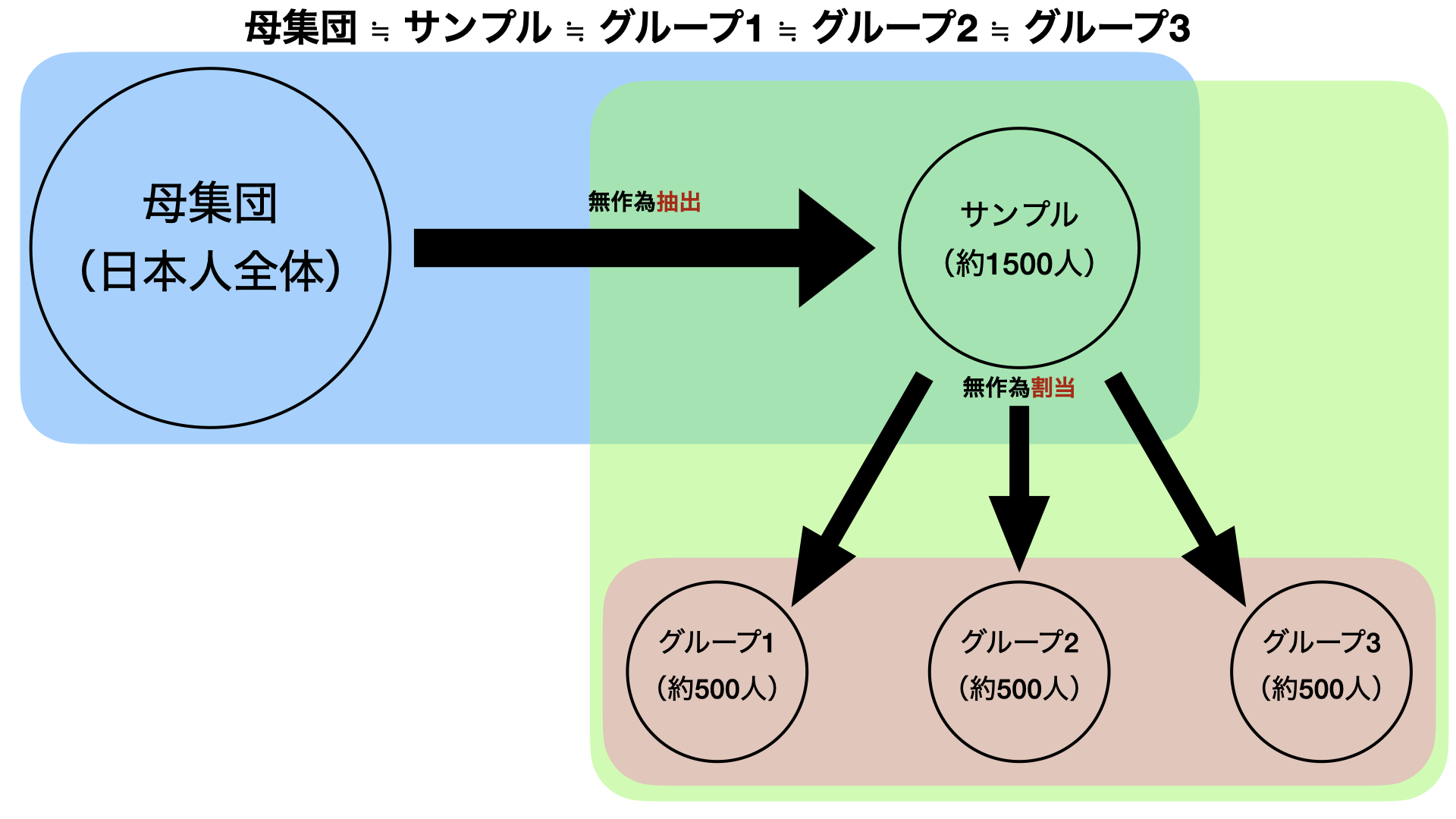
無作為抽出と無作為割当

• 無作為抽出によってサンプル（標本）と母集団が交換可能（実はここが難しい）
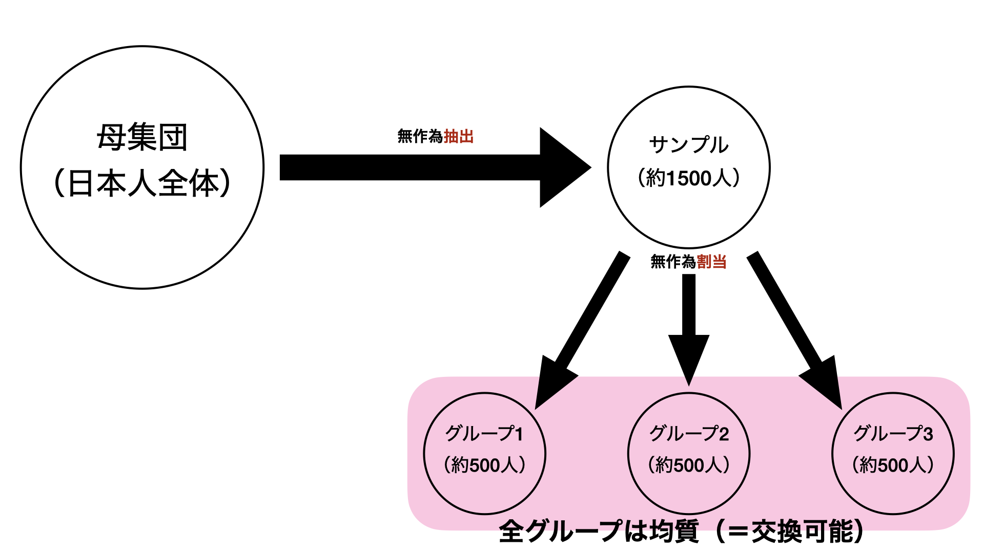
• 無作為割当によって各グループとサンプルに交換可能（=各グループ間で交換可能）
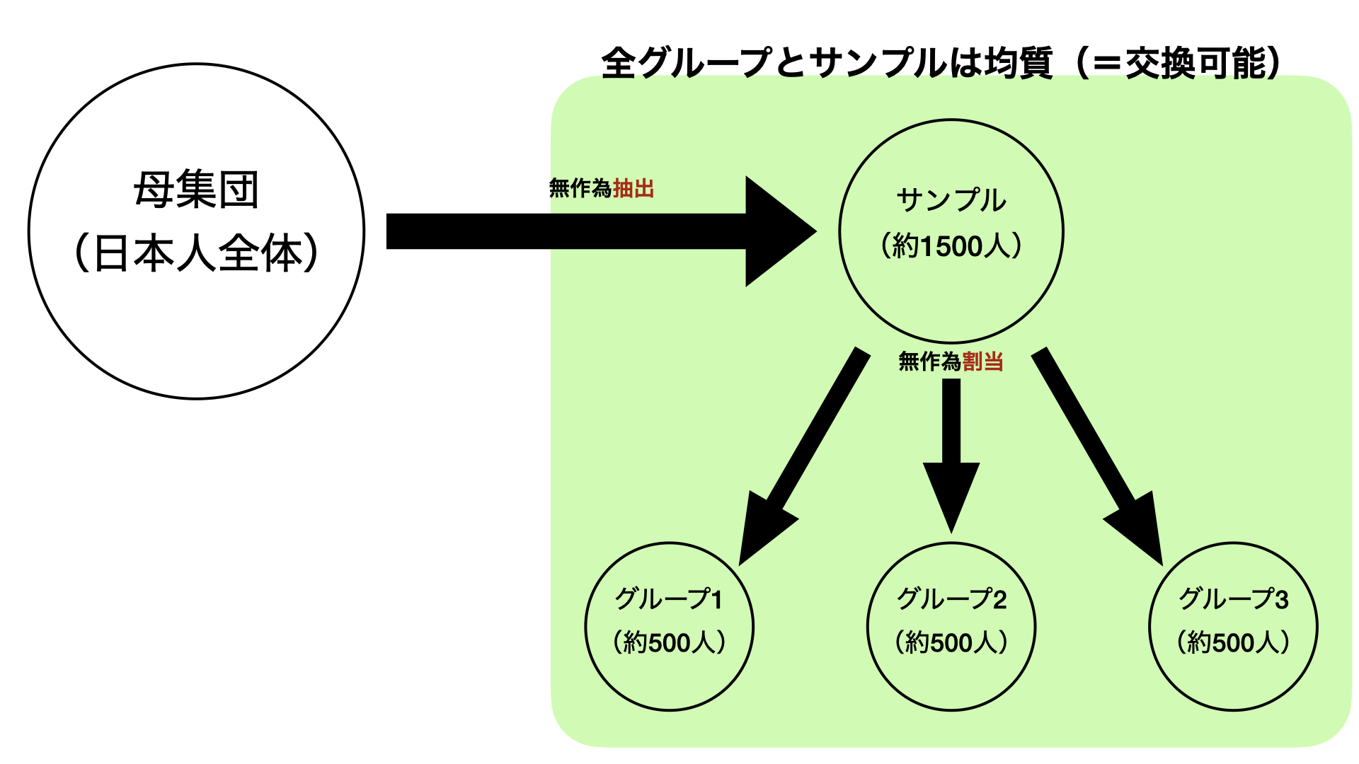
• 無作為抽出&無作為割当によって各グループと母集団が交換可能（グループへの刺激=母集団への刺激）

ランダム化比較試験

ランダム化比較試験とは

Randomized Controlled Trial（RCT）

• 無作為割当で複数のグループを作り上げた上で、異なる刺激・処置を与え、結果を観察する手法
  • 社会科学でいう「実験」の多くはこれを指す
  • 因果推論の王道
• 因果効果をもたらす（と想定される）処置変数が外生的
  • グループ間における結果変数の差 = 因果効果
• データ生成過程（Data Generating Process; DGP）への直接介入
  • 「真のモデル」が分かる

• 参考）データ生成過程について
  • 現実世界において、あるデータが生成されるプロセス
    • 例）\(Y\)は\(X_1\)と\(X_2\)の線形結合した値を平均値とする正規分布から生成される。
    • 例） \[ \begin{align} \hat{y} & \sim \mbox{Poisson}(\hat{\lambda}), \\ \hat{\lambda} & = e^{\beta_0 + \beta_1 X + \beta_2 Z}. \end{align} \]
  • King, Gary. 1989. Unifying Political Methodology, Michigan University Press.（Ch.1-4）
  • 豊田秀樹. 2022.『統計学入門 II: 尤度によるデータ生成過程の表現』朝倉書店

データ生成過程への介入

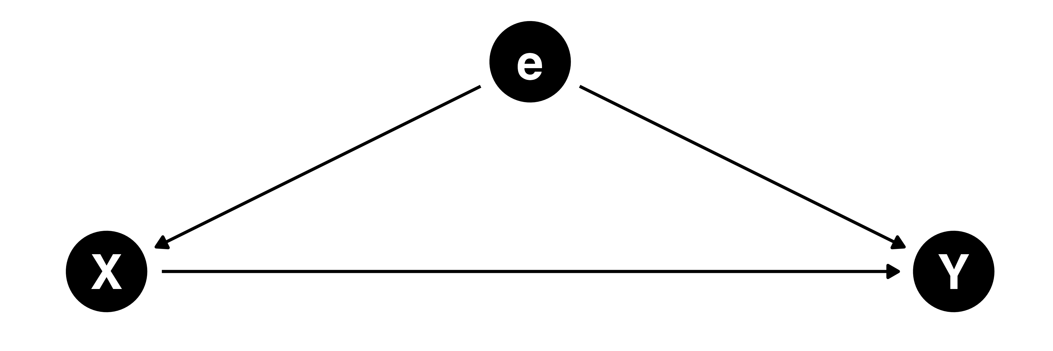
\[ \mbox{Income} = \beta_0 + \beta_1 \cdot \mbox{Quant} + \varepsilon \]

• Income：10年後の年収（\(\in [0, \infty)\)）
• Quant：ソンさんの講義を履修したか否か（\(\in \{0, 1\})\)）
• 誤差項(\(\varepsilon\))には「やる気」や「真面目さ」が含まれるため、Quantと相関がある（\(\rightarrow\) 内生性）
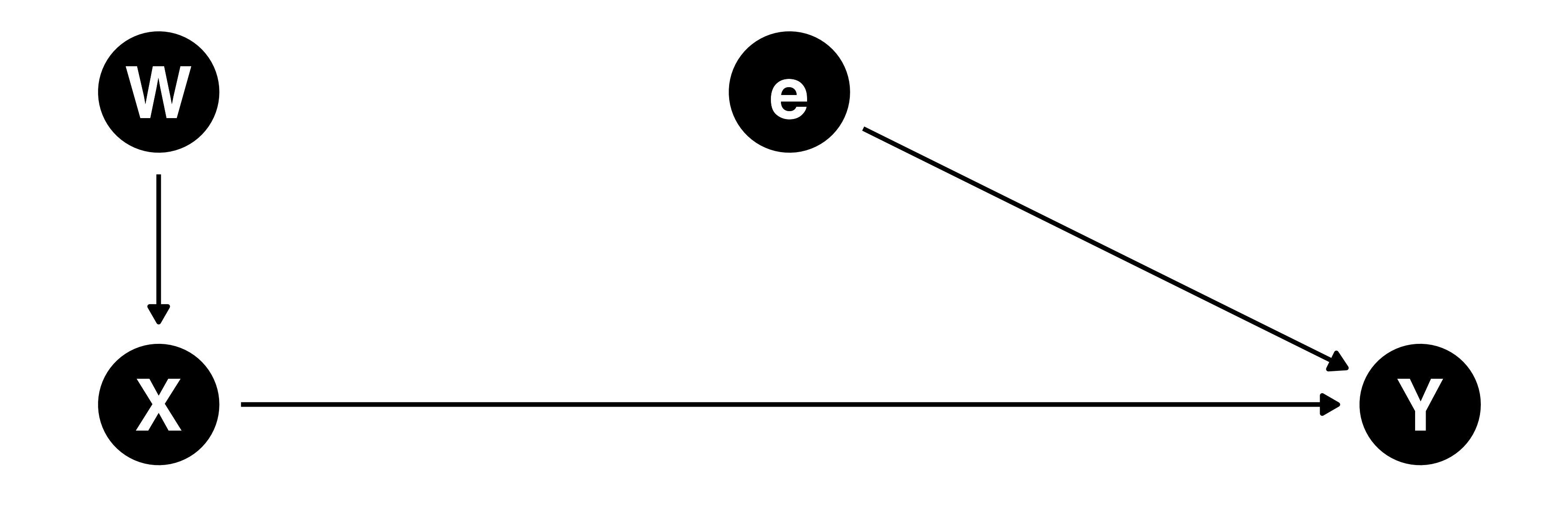
• 無作為割当で受講有無を決めると、「やる気」や「真面目さ」はQunatと無関係（独立）になる
  • 例) 受講有無をコイン投げ（\(W\)）で決める場合、コインの結果は誤差項（やる気や真面目さ）と独立（ただし、全員がコイン投げの結果に従うと仮定）
  • \(\Rightarrow\) 内生性がなくなる!

実験の方法

Hyde (2015) による分類

• フィールド実験: 実際の社会を舞台に行う実験
  • Gerber, Alan S. and Donald P. Green. 2012. Field Experiments, Norton.
• 実験室実験: 人為的に作られた（=統制された）環境内で行う実験
• サーベイ実験: 世論調査に埋め込む実験
  • SONG Jaehyun・秦正樹. 2020. 「オンライン・サーベイ実験の方法: 理論編」『理論と方法』35 (1): 92-108.
  • 秦正樹・SONG Jaehyun. 2020. 「オンライン・サーベイ実験の方法: 実践編」『理論と方法』35 (1): 109-127.

フィールド実験（1）

実際の社会を舞台に行う実験

• 例1
• 例2

Ito, Koichiro, Takanori Ida, and Makoto Tanaka. 2018. “Moral Suasion and Economic Incentives: Field Experimental Evidence from Energy Demand,” American Economic Journal: Economic Policy, 10 (1): 240-267.

• 京都府内の691世帯が対象
• 電気メーターを設置し、統制群と処置群1、処置群2に分割
  • 設置のみ (153) / 単純節電要請 (154) / 動機づけ節電要請 (384)
• 電気使用量の比較

Gerber, Alan S., Donald P. Green, and Christopher W. Larimer. 2010. “An Experiment Testing the Relative Effectiveness of Encouraging Voter Participation by Inducing Feelings of Pride or Shame,” Political Behavior, 32: 409-422.

• ミシガン州の18万世帯が対象
• 4つの処置群にそれぞれ異なる投票を促す内容の葉書を発送
  • 統制群: 99,999世帯 / 処置群1: 20,001世帯 / 処置群2: 20,002世帯 / 処置群3: 20,00 世帯 / 処置群4: 20,000世帯
• それぞれのグループ間の投票率を比較

フィールド実験（2）

• メリット
  • 実際の社会と対象にするため、高い外的妥当性
    • 一般的に外的妥当性は実験研究の最大の弱点とも言われる
    • ただし、全国民ではなく、一部の地域を対象にするケースが多いため、限界もある
      • Ito, Ida and Tanaka (2018) は外的妥当性の確保のために同様の実験を京都以外でも実施 (京都市、横浜市、北九州市、豊田市)
• デメリット
  • 高費用
    • Gerber, Green, and Larimer (2010) は安い方?
      • アメリカで切手は100円以上の場合が多いため、18万世帯$$100円だけでも1800万円
      • 葉書もタダじゃない (Amazon.comで100枚12ドル程度)
    • Ito, Ida and Tanaka (2018) は . . .
• 政府や企業などの協力なしでは実施が困難なケースが多い

実験室実験（1）

人為的に作られた環境内で行う実験

• 例1
• 例2

Blais, André, Simon Labbé-St-Vincent, Laslier Jean-François, Nicolas Sauger, and Karine Van der Straeten. 2011. “Strategic Vote Choice in One-Round and Two-Round Elections: An Experimental Study,” Political Research Quarterly, 64(3): 637–645.

• 42名 \(\times\) 2グループ
  • グループ1：一回投票制4回 \(\rightarrow\) 二回投票制4回
  • グループ2：二回投票制4回 \(\rightarrow\) 一回投票制4回
• 投票方式による戦略投票（Strategic Vote）の傾向を比較

Mueller, Pam A. and Daniel M. Oppenheimer. 2014. “The Pen Is Mightier Than the Keyboard: Advantages of Longhand Over Laptop Note Taking,” Psychological Science, 25(6): 1159-1168.

• 学生を2グループに分割
  • グループ 1: ノートパソコンでノートテイキング
  • グループ 2: ノートとペンでノートテイキング
• レクチャーの理解度をグループごとに比較

実験室実験（2）

• メリット
  • 環境を自由に操作できる
  • 被験者の訓練・統制が容易
    • 実験前のルールの説明など
• デメリット
  • 被験者の属性が偏りやすい \(\Rightarrow\) 低い外的妥当性
    • 主に学生が動員される
    • Hovland (1959): “College sophomores may not be people.”
• トレードオフ
  • 一般的に、被験者が少数
    • Small \(N\) \(\leftrightarrow\) 低コスト(単位を餌にする研究者ならタダでできる)

サーベイ実験（1）

世論調査に実験を埋め込む方法

• 例1
• 例2

Asaba, Yuki, Kyu S Hahn, Seulgi Jang, Tetsuro Kobayashi, and Atsushi Tago. 2020. “38 seconds above the 38th parallel: how short video clips produced by the US military can promote alignment despite antagonism between Japan and Korea,” International Relations of the Asia-Pacific, 20(2): 253–273.

• サーベイの回答者1500名を2グループに分割
  • 統制群：38秒の日米韓軍事協力に関するPACOM制作の動画を視聴
  • 処置群：ほぼ同じ長さのPACOM制作の動画を視聴（日韓の言及はなし）
• アメリカに対する感情温度、日韓協力に対する態度を測定
• グループごとに結果を比較

Song, Jaehyun, Takeshi Iida, Yuriko Takahashi, and Jesús Tovar. 2022. “Buying Votes across Borders? A List Experiment on Mexican Immigrants in the US,” Canadian Journal of Political Science, 55 (4): 852-872.

• 回答者621名を統制群と処置群に割当
• 統制群に以下のように質問

Now we are going to show you four activities that some people may experience during the electoral campaign. After you read all four, just answer HOW MANY activities you experienced during the last electoral campaign. (We do NOT want to know which ones, just how many.)

• I saw public debates between candidates for presidential elections on TV.
• I saw official websites/blogs of politicians and candidates.
• My family/friends told me about the election.
• Campaign activists threatened me to vote for a candidate.

• 処置群には「Campaign activists gave any monetary benefits or did a favor to me or my family in Mexico.」を追加
• 結果の平均値を比較

サーベイ実験（2）

• メリット
  • コストが低い (数万円で一応実施可能OK)
  • 大規模の実験が可能（数百人〜数千人）
  • 機動性が高い
  • SUTVA（後述）が満たされやすい
• デメリット
  • 実際の環境を再現するのが困難（外的妥当性の問題）
  • 「行動」を対象とした場合、測定尺度の問題
  • 不良回答者（satisficer）の存在
  • 実験のトラブルに対応するのが困難

RCTの例

Bertrand, Marianne, and Sendhil Mullainathan. 2004. “Are Emily and Greg More Employable Than Lakisha and Jamal? A Field Experiment on Labor Market Discrimination,” American Economic Review, 94(4): 991-1013.

• 労働市場における人種差別
• 約5000人分の架空の履歴書を求人中の会社へ送る
  • 履歴書の内容 (性別、人種、能力など) は完全無作為
  • 履歴書に人種は記入できないため、白人っぽい名前 (Emily など)、黒人っぽい名前 (Jamal など) を記入
• 後は、返事を待つだけ

処置変数: 人種 ( \(\in \{\text{black}, \text{white}\}\) )

結果変数: 連絡の有無 ( \(\in \{0, 1\}\) )

内生性の可能性

• 誤差項には教育水準、親の所得、居住地などが含まれる
  • 実際に人種と上記の要因には相関あり
  • 人種 (処置) と誤差項間の相関関係 \(\rightarrow\) 内生性
• 黒人が採用されなかった場合…
  • 黒人だから? \(\leftarrow\) 人種差別\(\bigcirc\)
  • 教育水準が低いから \(\leftarrow\) 人種差別\(\times\)

\(\Rightarrow\) 内生性がある限り、因果効果の識別は困難



\(\Rightarrow\) ケースによって政策的含意が変わる。

RCTの力

	白人の名前	黒人の名前
Female	76.42%	77.45%
HighQuality	50.23%	50.23%
Call Rate	9.65%	6.45%
計 (人)	2435	2435

• 無作為割当の結果、人種と性別・能力の相関がほぼ0に
  • 内生性のない状態
  • この場合、労働市場における人種の因果効果は
    • ATE = 黒人の平均連絡率 − 白人の平均連絡率
    • 黒人という理由だけで会社から連絡が来る確率が 3.2%p\(\downarrow\)
    • -3.2%p: 人種の因果効果 or 処置効果 (treatment effect)

バランスチェック

無作為割当が行われているか否かを確認

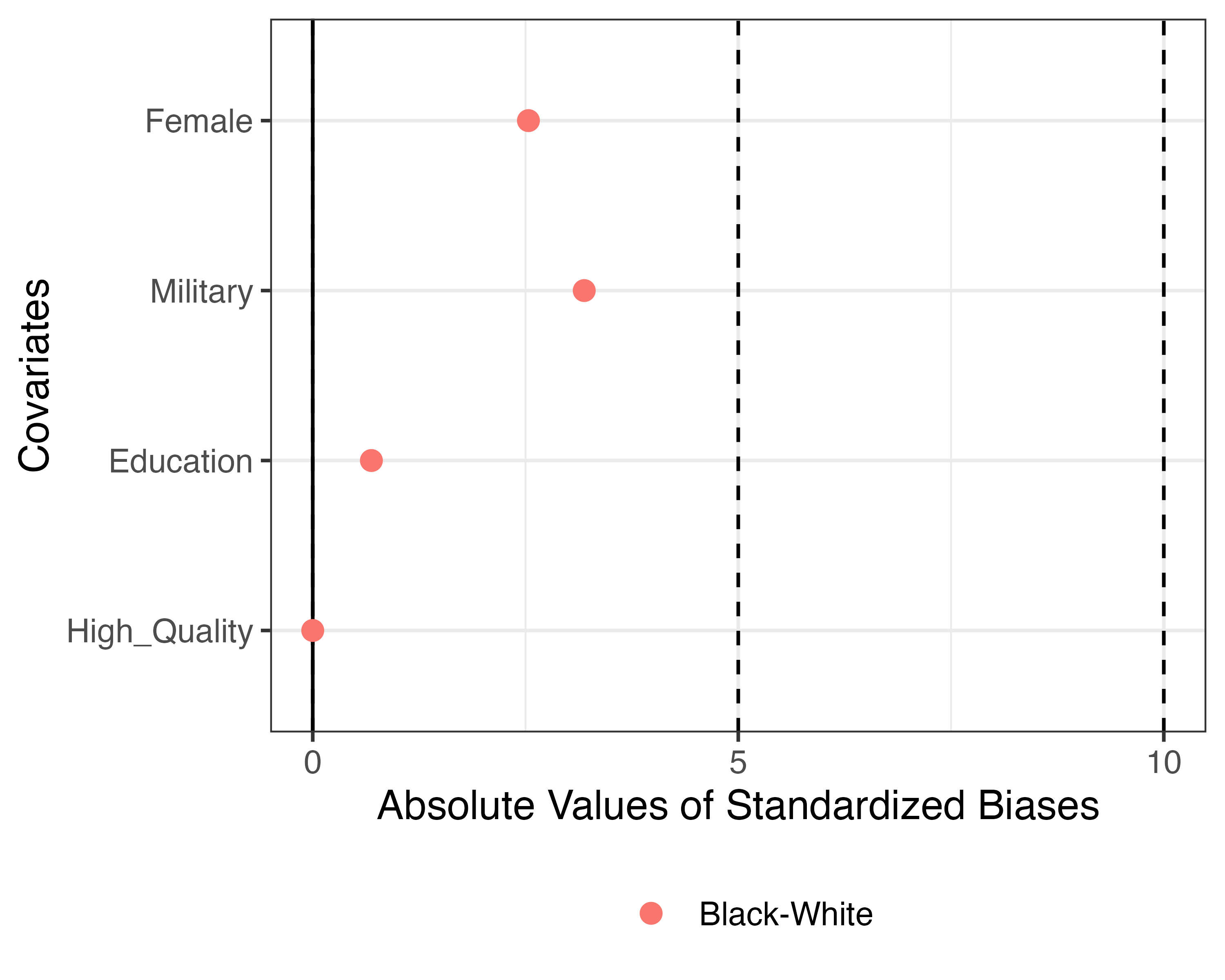
標準化差分を使用

• Standardized Bias (or Difference)
  • サンプルサイズの影響\(\times\)
  • 統計的検定ではない
• \(t\) 検定、ANOVA、 \(\chi^2\) 検定は\(\times\)
  • バランスチェックに統計的有意性検定は使わない
• {cobalt}、{BalanceR}など

標準化差分について

連続変数

\[ \text{SB}_{T-C} = 100 \cdot \frac{\bar{X}_T - \bar{X}_C}{\sqrt{0.5 \cdot (s_T^2 + s_C^2)}} \]

二値変数

\[ \text{SB}_{T-C} = 100 \cdot \frac{\bar{X}_T - \bar{X}_C}{\sqrt{0.5 \cdot (\bar{X}_T(1-\bar{X}_T) + \bar{X}_C(1-\bar{X}_C))}} \]

• \(\bar{X}_T\) : 処置群におけるXの平均値
• \(s_T^2\) : 処置群におけるXの分散
• |SB|が小さいほどバランス
  • 明確な基準はないが、3、5、10、25などを使用
• グループが3つ以上の場合、それぞれのペアで実行

因果効果の推定

• 平均値の差分の検定
• 単回帰分析

方法1: グループ間の結果変数の差分の検定 (\(t\)検定)

• 因果効果 (ATE): \(\mathbb{E}[\mbox{Call}|\mbox{Race = Black}] - \mathbb{E}[\mbox{Call}|\mbox{Race = White}] = -0.032\)
• ATE = 0の帰無仮説の検定
  • \(t_{\text{df} = 4711.7} = −4.117\); \(p\) < 0.001; 95% CI = [−0.047, −0.017]
• 応答変数の尺度に応じてノンパラメトリック分析

方法2: 単回帰分析 (線形 or ロジスティックス/プロビット)

線形回帰分析（LPM）

Covriates	Est.	S.E.
Intercept	0.064	0.006
Race: White	0.032	0.008

ロジスティック回帰分析

Covriates	Est.	S.E.
Intercept	-2.675	0.083
Race: White	0.438	0.107

プロビット回帰分析

Covriates	Est.	S.E.
Intercept	-1.518	0.039
Race: White	0.217	0.053

参考）Freedman, David A. 2008. “Randomization Does Not Justify Logistic Regression,” Statistical Science Statistical Science, 23(2): 237-249.

• Logit: 一致推定量\(\times\) & 不偏推定量\(\times\)
• Linear: 一致推定量\(\bigcirc\) & 不偏推定量\(\times\)
• 一致性と不偏性の違いについて

因果効果の推定：重回帰分析は?

無作為割当のおかげですべての変数が互いに独立

• 重回帰分析をしても人種のATEは変化しない (OVB がない)
  • 無作為割当の場合、回帰はしてもしなくても良い
• 現実的に完全にバランスが取れていないため、若干の変化はある

Covriates	Est.	S.E.
Intercept	0.057	0.007
Race: White	0.032	0.08
Female	0.007	0.009
Military	-0.027	0.014
Education	-0.002	0.005
High Quality	0.019	0.008

因果効果の不均一性

因果効果が下位グループによって異なる場合

• 因果効果の不均一性 (heterogeneous treatment effects)
  • 例) 性別によって薬の効果が異なる場合
  • 薬の効果が男性なら 1、女性なら 2 の場合
    • 男女比が1:1なら、ATEは1.5に
  • 薬の効果が男性なら 4、女性なら-1 の場合
    • 男女比が1:1なら、ATEは1.5だが…
• 方法1: 男女に分けてATEを推定
• 方法2: 性別と処置有無の交差項を投入した重回帰分析

参考) Bryan, Christopher J., Elizabeth Tipton and David S. Yeager. 2021. “Behavioural science is unlikely to change the world without a heterogeneity revolution,” Nature Human Behaviour. 5: 980–989.

因果効果の不均一性（intro_data2.csv）

data2 <- read_csv("data/intro_data2.csv")

data2

# A tibble: 500 × 4
      ID Outcome Treatment Female
   <dbl>   <dbl>     <dbl>  <dbl>
 1     1  1.09           0      1
 2     2  0.0281         0      1
 3     3  1.65           0      0
 4     4  3.83           1      1
 5     5  2.65           1      1
 6     6  1.24           1      1
 7     7  0.136          1      0
 8     8  0.507          0      1
 9     9  2.99           1      1
10    10  4.34           1      1
# ℹ 490 more rows

因果効果の不均一性

方法1: 男女に分けてATEを推定

• 比較
• コード1
• コード2
• コード3

	統制群	処置群	ATE	\(t\)	\(p\)
男性のみ	0.611	1.561	0.951	-7.521	< 0.001
女性のみ	0.493	2.480	1.987	-15.573	< 0.001
全体	0.551	2.057	1.506	-15.945	< 0.001

男性のみ

t.test(Outcome ~ Treatment, data = data2, subset = (Female == 0))

    Welch Two Sample t-test

data:  Outcome by Treatment
t = -7.5211, df = 235.95, p-value = 1.132e-12
alternative hypothesis: true difference in means between group 0 and group 1 is not equal to 0
95 percent confidence interval:
 -1.1996845 -0.7016501
sample estimates:
mean in group 0 mean in group 1 
      0.6105137       1.5611810 

女性のみ

t.test(Outcome ~ Treatment, data = data2, subset = (Female == 1))

    Welch Two Sample t-test

data:  Outcome by Treatment
t = -15.573, df = 259.72, p-value < 2.2e-16
alternative hypothesis: true difference in means between group 0 and group 1 is not equal to 0
95 percent confidence interval:
 -2.238053 -1.735599
sample estimates:
mean in group 0 mean in group 1 
      0.4931905       2.4800169 

全体

t.test(Outcome ~ Treatment, data = data2)

    Welch Two Sample t-test

data:  Outcome by Treatment
t = -15.945, df = 494.24, p-value < 2.2e-16
alternative hypothesis: true difference in means between group 0 and group 1 is not equal to 0
95 percent confidence interval:
 -1.692061 -1.320817
sample estimates:
mean in group 0 mean in group 1 
      0.5509135       2.0573524 

因果効果の不均一性

方法2: 性別と処置有無の交差項を投入した重回帰分析

lm(Outcome ~ Treatment * Female, 
   data = data2) |>
   summary()

	(1)
(Intercept)	0.611 (0.091)
Treatment	0.951 (0.131)
Female	-0.117 (0.127)
Treatment × Female	1.036 (0.180)
Num.Obs.	500
R2 Adj.	0.398
F	110.905

\[ \begin{align} \hat{y} = & \beta_0 + \beta_1 \mbox{Treatment} + \beta_2 \mbox{Female} + \\ & \beta_3 \mbox{Treatment} \cdot \mbox{Female} \\ = & \beta_0 + (\beta_1 + \beta_3 \mbox{Female}) \mbox{Treatment} + \beta_2 \mbox{Female}. \end{align} \]

• 処置効果はTreatmentの係数
  • \(\beta_1 + \beta_3 \mbox{Female}\)
  • \(\Rightarrow\) 処置効果がFemaleの値にも依存
• 男性のATE: \(\beta_1 + \beta_3 \cdot 0 = \beta_1\) = 0.951
• 女性のATE: \(\beta_1 + \beta_3 \cdot 1 = \beta_1 + \beta_3\) = 1.987

因果推論の前提:SUTVA

Stable Unit Treatment Value Assumption

• 非干渉性
• 処置の無分散性
• サーベイ実験の場合

非干渉性: 他人の処置・統制有無が処置効果に影響を与えないこと

• 例) AさんITEは
  • 例1) Bさんが統制群の場合は10、処置群の場合は5 \(\leftarrow\)
  • 例2) Bさんが統制群の場合も、処置群の場合も、5 \(\leftarrow\)

例1

	Aさんが統制群	Aさんが処置群
Bさんが統制群	0	10
Bさんが処置群	15	20

例2

	Aさんが統制群	Aさんが処置群
Bさんが統制群	5	10
Bさんが処置群	15	20

処置の無分散性: 同じグループに属する対象は同じ処置を受けること

• 手術の場合：医者、設備、手順、環境など
• 投票参加：当日、期日前など

• サーベイ実験ではSUTVAが満たされやすい。
  • 実験室実験、フィールド実験の場合、「非干渉性」には気をつける。
  • 例) 隣の人が見てるのとと私が見てるのが違いますが…?

二重盲検法

二重盲検法（Double Blind Test）：ある被験者がどのような処置を受けているかについて研究者と被験者両方において不明な状態で実験を行うこと

二重盲検法を使えば以下の問題点に対処することが可能

• プラセボ効果（placebo effect）：偽薬が与えられても、薬だと信じ込む 事によって何らかの効果が生じる
• ホーソン効果（Hawthorne effect）：自分が観察されていることを認知さ れることによって何らかの効果が生じる
• 観察者効果（observer/experimenter effect）：研究者の期待により被験者へ の対応が異なったり、被験者がその期待に添えるように行動すること

来週以降の実習について

用意するもの

第4、5、6回はRの実習

• ノートPC
  • デスクトップ、モニター、キーボード、マウスが持ち込めるなら、デスクトップでもOK（がんばって！！）
• Rの導入（いずれの方法でもOK）
  • 自分のPCにR/RStudioをインストールし使用する。
  • JDCat分析ツール（クラウド版のR + RStudio）を使用する。
• ブラインドタッチ